Introduction to complexity

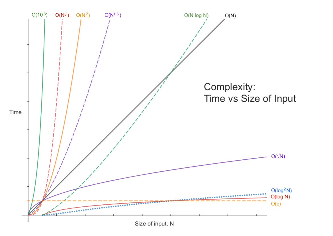
We write computer programs to perform calculations and solve problems, and we can measure the “complexity” of each program or algorithm we implement. Most commonly we talk about how the run time of an algorithm changes with the size of its input. If it takes y amount of time when we have input of size x, what happens if we increase the size of the input to 2x? Does the run time double? Does it increase more quickly? More slowly?
These are crucial questions for understanding the efficiency of our algorithms and often gives us some theoretical limit.
Here are two videos that introduce the topic of complexity (7:26 and 12:59).
Part 1: Basics and Asymptotic Notation
Part 2: Examples and Calculations
Is quadratic time complexity OK?
What do you think? Is \mathcal{O}(n^2) “pretty good”? Nowadays, computers have a lot of memory which means they can work on bigger problems than they could back in the olden days. What if you had an algorithm that had \mathcal{O}(n^2) complexity and took 10 microseconds per operation? With 100 records, that’s 100 x 100 x 10 = 100,000 microseconds, or 0.1 seconds. So far so good. What if you had 1,000 records? Your algorithm would take 10 seconds to run. Not too bad, right? What if you had a million records (not at all implausible). You’d need 10^6 \times 10^6 \times 10 = 10^{13} seconds—that’s over 300,000 years! So \mathcal{O}(n^2) is only suitable for small problem instances. In most applications, \mathcal{O}(n^2) is unacceptable.
More to consider
Once you’ve watched both videos, think about how you would approach a problem knowing that the theoretical limit for an algorithm was \mathcal{O}(n \log n), but your code had \mathcal{O}(n^2) complexity. What would you do?
In a very different scenario, what if you knew that the best known algorithm were on the order of \mathcal{O}(n^2) but you had a huge data set to process? What then? (This is one kind of question we address in CS 3240 Algorithm Design and Analysis.)
See also: Essential Algorithms, chapter 1, for more on complexity and asymptotic notation.
Resources
Additional reading
Comprehension check
- True or false? When performing asymptotic analysis we give special emphasis on constants and leading coefficients.
- In a polynomial, the term with the largest exponent is a ______________________ term.
- Big O gives a(n) _______________ bound on complexity.
- Simple arithmetic calculations occur in ________________ time.
- Iterating through a 2D array and performing a calculation on array elements takes two nested loops and therefore has ______________ complexity.
- True or false? An \mathcal{O}(n \log n) algorithm is more efficient than an \mathcal{O}(\sqrt{n}) algorithm that performs the same calculation.
- True or false? An \mathcal{0}(n^{1.5}) algorithm is more efficient than an \mathcal{O}(n \log n) algorithm that performs the same calculation.
Answers: ǝslɐɟ[ / ]ǝslɐɟ / (ᄅ^u)O / ɹɐǝuᴉl / ɹǝddn / ƃuᴉʇɐuᴉɯop / ǝslɐɟ
Copyright © 2023–2025 Clayton Cafiero
No generative AI was used in producing this material. This was written the old-fashioned way.