
Mixed Models for Missing Data
With Repeated Measures Part 1
David C. Howell

This is a two part document. For the second part go to
Mixed-Models-for-Repeated-Measures2.html. I have another document at Mixed-Models-Overview.html, which has much of the same material, but with a somewhat different focus.
When we have a design in which we have both random and fixed variables, we have what is often called a mixed model. Mixed models have begun to play an important role in statistical analysis and offer many advantages over more traditional analyses. At the same time they are more complex and the syntax for software analysis is not always easy to set up. I will break this paper up into two papers because there are a number of designs and design issues to consider. This document will deal with the use of what are called mixed models (or linear mixed models, or hierarchical linear models, or many other things) for the analysis of what we normally think of as a simple repeated measures analysis of variance.
A large portion of this document has benefited from Chapter 15 in Maxwell & Delaney (2004) Designing Experiments and Analyzing Data. They have one of the clearest discussions that I know. I am going a step beyond their example by including a between-groups factor as well as a within-subjects (repeated measures) factor. For the moment my purpose is to show the relationship between mixed models and the analysis of variance. The relationship is far from perfect, but it gives us a known place to start. More importantly, it allows us to see what we gain and what we lose by going to mixed models. Maxwell & Delaney based their analyses on SAS. I originally did that, but decded that SPSS was a better approach for most people. The result are nearly indistinquishable. I will also include R code, though it is somewhat more difficult to understand.
My motivation for this document came from a question asked by Rikard Wicksell at Karolinska University in Sweden. He had a randomized clinical trial with two treatment groups and measurements at pre, post, 3 months, and 6 months. His problem is that some of his data were missing. He considered a wide range of possible solutions, including "last trial carried forward," mean substitution, and listwise deletion. In some ways listwise deletion appealed most, but it would mean the loss of too much data. One of the nice things about mixed models is that we can use all of the data we have. If a score is missing, it is just missing. It has no effect on other scores from that same patient.
Another advantage of mixed models is that we don't have to be consistent about time. For example, and it does not apply in this particular example, if one subject had a follow-up test at 4 months while another had their follow-up test at 6 months, we simply enter 4 (or 6) as the time of follow-up. We don't have to worry that we couldn't measure all patients at the same intervals.
A third advantage of these models is that we do not have to assume sphericity or compound symmetry in the model. We can do so if we want, but we can also allow the model to select its own set of covariances or use covariance patterns that we supply. I will start by assuming sphericity because I want to show the parallels between the output from mixed models and the output from a standard repeated measures analysis of variance. I will then delete a few scores and show what effect that has on the analysis. I will compare the standard analysis of variance model with a mixed model. Finally I will use Expectation Maximization (EM) and Multiple Imputation (MI) to impute missing values and then feed the newly complete data back into a repeated measures ANOVA to see how those results compare. (If you want to read about those procedures, I have a web page on them at Missing.html).
The Data
I have created data to have a number of characteristics. There are two groups - a Control group and a Treatment group, measured at 4 times. These times are labeled as 1 (pretest), 2 (one month posttest), 3 (3 months follow-up), and 4 (6 months follow-up) -- or, in some cases, 0, 1, 3, 6. I created the treatment group to show a sharp drop at post-test and then sustain that drop (with slight regression) at 3 and 6 months. The Control group declines slowly over the 4 intervals but does not reach the low level of the Treatment group. There are noticeable individual differences in the Control group, and some subjects show a steeper slope than others. This last fact will become important in creating a covariance matrix that does not show compound symmetry.) In the Treatment group there are individual differences in level but the slopes are not all that much different from one another. You might think of this as a study of depression, where the dependent variable is a depression score (e.g. Beck Depression Inventory) and the treatment is drug versus no drug. If the drug worked about as well for all subjects the slopes would be comparable and negative across time. For the control group we would expect some subjects to get better on their own and some to stay depressed, which would lead to differences in slope for that group. These facts are important because when we get to the random coefficient mixed model the individual differences will show up as variances in intercept, and any slope differences will show up as a significant variance in the slopes. For the standard ANOVA, and for the SPSS mixed models, the differences in level show up as a Subject effect and we assume that the slopes are comparable across subjects.
The program and data used below are available at the following links. I explain below the differences between the data files. For the data with missing cases, I have used "999" as the missing data code.
WicksellWideComplete.dat
WicksellLongComplete.dat
WicksellWideMiss.dat
WicksellLongMiss.dat
The data follow. Notice that to set this up for a standard repeated measures ANOVA we read in the data one subject at a time. (You can see this in the data shown. Files like this are often said to be in "wide format" for reasons that are easy to see.) This will become important because we will not do that for mixed models. There we will use the "long" format.
| Group |
Subj |
Time0 |
Time1 |
Time3 |
Time6 |
| 1 |
1 |
296 |
175 |
187 |
192 |
| 1 |
2 |
376 |
329 |
236 |
76 |
| 1 |
3 |
309 |
238 |
150 |
123 |
| 1 |
4 |
222 |
60 |
82 |
85 |
| 1 |
5 |
150 |
271 |
250 |
216 |
| 1 |
6 |
316 |
291 |
238 |
144 |
| 1 |
7 |
321 |
364 |
270 |
308 |
| 1 |
8 |
447 |
402 |
294 |
216 |
| 1 |
9 |
220 |
70 |
95 |
87 |
| 1 |
10 |
375 |
335 |
334 |
79 |
| 1 |
11 |
310 |
300 |
253 |
140 |
| 1 |
12 |
310 |
245 |
200 |
120 |
| 2 |
13 |
282 |
186 |
225 |
134 |
| 2 |
14 |
317 |
31 |
85 |
120 |
| 2 |
15 |
362 |
104 |
144 |
114 |
| 2 |
16 |
338 |
132 |
91 |
77 |
| 2 |
17 |
263 |
94 |
141 |
142 |
| 2 |
18 |
138 |
38 |
16 |
95 |
| 2 |
19 |
329 |
62 |
62 |
6 |
| 2 |
20 |
292 |
139 |
104 |
184 |
| 2 |
21 |
275 |
94 |
135 |
137 |
| 2 |
22 |
150 |
48 |
20 |
85 |
| 2 |
23 |
319 |
68 |
67 |
12 |
| 2 |
24 |
300 |
138 |
114 |
174 |
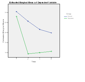
The means and a plot of the data follows:
Descriptive Statistics
			Group		Mean	Std. Deviation	N
Time0			Control		304.33	79.064		12
			Treatment	280.42	69.611		12
			Total		292.38	73.868		24
Time1			Control		256.67	107.850		12
			Treatment	94.50	47.565		12
			Total		175.58	116.213		24
Time3			Control		215.75	76.504		12
			Treatment	100.33	57.975		12
			Total		158.04	88.779		24
Time6			Control		148.83	71.287		12
			Treatment	106.67	55.794		12
			Total		127.75	66.205		24
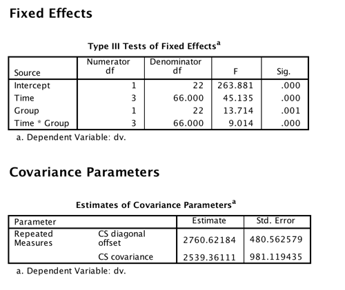
The abbreviated results of a standard repeated measures analysis of variance with no missing data and using SPSS General Linear Model/Repeated Measures follow.
Tests of Within-Subjects Effects
Measure:   MEASURE_1
Source		               Type III Sum of Squares	df	Mean Square	F      Sig.
Time	        Sphericity Assumed	373802.708	3	124600.903    45.135   .000

Time * Group	Sphericity Assumed	74654.250	         24884.750     9.014   .000
		Greenhouse-Geisser	74654.250	2.189	 34104.770     9.014   .000

Error(Time)	Sphericity Assumed	182201.042	66	2760.622
		Greenhouse-Geisser	182201.042	48.157	3783.457

_______________________________________________________________________________________

Tests of Between-Subjects Effects
Measure:   MEASURE_1
Transformed Variable:   Average

Source	      Type III Sum of Squares	df	Mean Square	F	Sig.
   Intercept	     3408834.375	 1	3408834.375	263.881	.000
   Group	     177160.167	         1	 177160.167	13.714	.001
   Error	     284197.458	        22	  12918.066
Toggle triangle to see R code
# Notice that the data are read in the long form.
library(car)
setwd("~/Dropbox/Webs/StatPages/Mixed-Models-Repeated")
data2 <- read.table("WicksellLongComplete.dat", header = TRUE)
head(data2)
####################################################################
 head(data)
#   Subj Time Group  dv
#    1    0     1 296
#    1    1     1 175
#    1    3     1 187
#    1    6     1 192
#    2    0     1 376
#    2    1     1 329
####################################################################
data2$Group <- factor(data2$Group)  #I don't like to use 'attach'.
data2$Subj <- factor(data2$Subj)
data2$time.cont <- data2$Time
data2$Time <- factor(data2$Time)
### Using aov
Wicksellaov <- aov(dv~Group*Time + Error(Subj), data = data2)
print(summary(Wicksellaov))
_________________________________________

Error: Subj
          Df Sum Sq Mean Sq F value  Pr(>F)
Group      1 177160  177160   13.71 0.00124 **
Residuals 22 284197   12918


Error: Within
           Df Sum Sq Mean Sq    F value   Pr(>F)
Time        3 373803  124601  45.135 5.55e-16 ***
Group:Time  3  74654   24885   9.014 4.38e-05 ***
Residuals  66 182201    2761

_______________________________________________

Tests of Within-Subjects Contrasts
Measure:   MEASURE_1
Source  Time Sum Squares df    Mean Square        F      Sig.
Time
    Linear 313856.408     1	313856.408	68.424	.000
    Quad    44893.500     1	 44893.500	18.147	.000
    Cubic   15052.800     1	 15052.800	12.328	.002
Time * Group
    Linear     19.200     1	    19.200	.004	.949
    Quad    67098.375     1	 67098.375	27.122	.000
    Cubic    7536.675     1	  7536.675	6.173	.021
Error(Time)
    Linear  100912.792   22	  4586.945
    Quad     54426.125   22	  2473.915
    Cubic    26862.125   22	  1221.006
If you toggle the analyses in R, you will see that they are exactly the same. But notice that we are using the standard analysis of variance solution here.
I should mention at this point that using R is far more complicated than using SPSS. I like R, but the discussions around mixed models in R are far from simple, and they often leave you with more questions than they answer. I will show the R output for several of the analyses, but I must say that if you gave me a set of data for analysis, I would be more likely to fall back on SPSS or SAS. I would feel that I have more control over setting up a model that I understand.
For this analysis we see that each of the effects in the overall analysis is significant. We don't care very much about the Group effect because we expected both groups to start off equal at pre-test. Similarly, we don't care much about the Time effect, because the interaction shows us that there is a different time effect in each group. By-and-large, when you have a significant interaction the main effects are usually unimportant unless you have a very specific reason for attending to them. What is important is the interaction, and it is significant at p = .0001. Clearly the drug treatment is having a differential effect on the two groups, which is what we wanted to see. The fact that the Control group seems to be dropping in the number of symptoms over time is to be expected and not exciting, although we could look at these simple effects if we wanted to. We would just run two analyses, one on each group. I would not suggest pooling the variances to calculate F, though that would be possible. I should mention that if you ran this analysis using R and its mixed model library (lme4), you would obtain the same results, but that is because this is a balanced design with no missing data. You can see that analysis if you go to Mixed-Models-Overview.html.
There are two different major approaches to mixed models in R, although they were both primarily authored by Douglas Bates and his colleagues. The first one is named nlme, while the second is named lme4. Neither of these is simple to use for a complex case, though nlme will allow you to specify different forms of the variance covariance matrix. (There have been promises for a long time that this capability will be added to lme4, but those who have been holding their breath for that have long since passed out.) If you toggle the following link, you will see that in this case lme4 produces the same result as above.
Toggle triangle to see R code using lme4
 The following F values are the same, but note that the SS for Group is different.
> Wickselllm <- lmer(dv ~ Group*Time + (1|Subj), data = data2 )
> anova(Wickselllm)
Analysis of Variance Table
           Df Sum Sq Mean Sq F value
Group       1  37860   37860 13.7141
Time        3 373803  124601 45.1351
Group:Time  3  74654   24885  9.0142
Mixed Model
The use of mixed models represents a substantial difference from the traditional analysis of variance. For balanced designs (which roughly translates to equal cell sizes) the results will come out to be the same, assuming that we set the analysis up appropriately. But the actual statistical approach is quite different and ANOVA and mixed models will lead to different results whenever the data are not balanced or whenever we try to use different, and often more logical, covariance structures.
But why amI talking about mixed models when I was supposed to be talking about repeated measures?
Mixed models deal with the case where some of your independent variables are random variables and some are fixed. In a repeated measures designs, we have multiple measures from the same subject. That means that we will need a term for Subjects, and in almost all practical examples, subjects are a random factor while Groups and Trials are fixed. Hence we have a mixed model.
By definition, mixed models involve both fixed and random independent variables. You might expect that we would have developed nice clear distinctions between fixed and random effects, but we haven't. In general a fixed variable includes all of the levels of that variable that you care about. Instead of selecting levels randomly from some possible population of levels, we choose them very deliberately and intend to interpret our results within the levels we have used. An example might be 3 different antidepressant drugs or 5 different levels of one drug. Gender is always a fixed variable because we if we are comparing genders we only have two genders to work with.
A random variable, on the other hand, is thought to be chosen from a population of levels. If, for example, we want to see how people identify letters, we could randomly choose 6 letters from the alphabet. If we repeated this study we would probably come up with 6 different letters. And we want to interpret our results with respect to the whole population of (26) possible letters. Similarly we might randomly choose classrooms or schools from all possible schools in California. Again, we want our results to generalize to at least California schools in general, not just the ones we used. When we are dealing with random variables, our primary interest is not in the differences between school-A and school-B, for example, but in the variance of school performance.
Covariance Structures
First a bit of theory. You should recall that for a standard repeated measures analysis of variance we assume that the covariance matrix meets our sphericity assumption and we go from there. In other words the calculations are carried out with the covariance matrix forced to sphericity. If that is not a valid assumption we are in trouble. Of course there are corrections due to Greenhouse and Geisser and Hyunh and Feldt, but they are not optimal solutions.
But what does compound symmetry, or sphericity, really represent? (The assumption is really about sphericity, but when speaking of mixed models most writers refer to compound symmetry, which is actually a bit more restrictive.) Most people know that compound symmetry means that the pattern of covariances or correlations is constant across trials. In other words, the correlation between trial 1 and trial 2 is equal to the correlation between trial 1 and trial 4 or trial 3 and trial 4, etc. But a more direct way to think about compound symmetry is to say that it requires that all subjects in each group change in the same way over trials. In other words the slopes of the lines regressing the dependent variable on time are the same for all subjects. Put that way it is easy to see that compound symmetry can really be an unrealistic assumption. If some of your subjects improve but others don't, you do not have compound symmetry and you make an error if you use a solution that assumes that you do. Fortunately SPSS Mixed Models and R's nlme, allow you to specify some other pattern for those covariances.
We can also get around the sphericity assumption using the the SPSS multivariate model, often called Manova, procedure, but that too has its problems. Both standard univariate GLM and MANOVA GLM will insist on complete data. If a subject is missing even one piece of data, that subject is discarded. That is a problem because with a few missing observations we can lose a great deal of data and degrees of freedom.
The Mixed-Models procedure is different. Instead of using a least squares solution, which requires complete data, it uses a maximum likelihood solution, which does not make that assumption. (We will often use a Restricted Maximum Likelihood (REML) solution.) When we have balanced data both least squares and REML will produce the same solution if we specify a covariance matrix with compound symmetry. But even with balanced data if we specify some other covariance matrix the solutions will differ. At first I am going to force sphericity by specifying that I want to assume that the covariance structure has compound symmetry. I will later relax that structure.
Data in the "Long Form"
The first analysis below uses exactly the same complete data as the previous analysis, though they are entered differently. Here data are entered in what is called "long form," as opposed to the "wide form" used for standard Anova. This means that instead of having one line of data for each subject, we have one line of data for each observation. So with four measurement times we will have four lines of data for that subject. I have put the data in three columns to save space, but the real syntax statements would have 96 lines of data. (This is what we used in the R solution given above.) A preliminary analysis follows.
| Subj Time Group dv
1 0 1.00 296.00
1 1 1.00 175.00
1 3 1.00 187.00
1 6 1.00 192.00
2 0 1.00 376.00
2 1 1.00 329.00
2 3 1.00 236.00
2 6 1.00 76.00
3 0 1.00 309.00
3 1 1.00 238.00
3 3 1.00 150.00
3 6 1.00 123.00
4 0 1.00 222.00
4 1 1.00 60.00
4 3 1.00 82.00
4 6 1.00 85.00
5 0 1.00 150.00
5 1 1.00 271.00
5 3 1.00 250.00
5 6 1.00 216.00
6 0 1.00 316.00
6 1 1.00 291.00
6 3 1.00 238.00
6 6 1.00 144.00
7 0 1.00 321.00
7 1 1.00 364.00
7 3 1.00 270.00
7 6 1.00 308.00
8 0 1.00 447.00
8 1 1.00 402.00
8 3 1.00 294.00
8 6 1.00 216.00
|
9 0 1.00 220.00
9 1 1.00 70.00
9 3 1.00 95.00
9 6 1.00 87.00
10 0 1.00 375.00
10 1 1.00 335.00
10 3 1.00 334.00
10 6 1.00 79.00
11 0 1.00 310.00
11 1 1.00 300.00
11 3 1.00 253.00
11 6 1.00 140.00
12 0 1.00 310.00
12 1 1.00 245.00
12 3 1.00 200.00
12 6 1.00 120.00
13 0 2.00 282.00
13 1 2.00 186.00
13 3 2.00 225.00
13 6 2.00 134.00
14 0 2.00 317.00
14 1 2.00 31.00
14 3 2.00 85.00
14 6 2.00 120.00
15 0 2.00 362.00
15 1 2.00 104.00
15 3 2.00 144.00
15 6 2.00 114.00
16 0 2.00 338.00
16 1 2.00 132.00
16 3 2.00 91.00
16 6 2.00 77.00
|
17 0 2.00 263.00
17 1 2.00 94.00
17 3 2.00 141.00
17 6 2.00 142.00
18 0 2.00 138.00
18 1 2.00 38.00
18 3 2.00 16.00
18 6 2.00 95.00
19 0 2.00 329.00
19 1 2.00 62.00
19 3 2.00 62.00
19 6 2.00 6.00
20 0 2.00 292.00
20 1 2.00 139.00
20 3 2.00 104.00
20 6 2.00 184.00
21 0 2.00 275.00
21 1 2.00 94.00
21 3 2.00 135.00
21 6 2.00 137.00
22 0 2.00 150.00
22 1 2.00 48.00
22 3 2.00 20.00
22 6 2.00 85.00
23 0 2.00 319.00
23 1 2.00 68.00
23 3 2.00 67.00
23 6 2.00 12.00
24 0 2.00 300.00
24 1 2.00 138.00
24 3 2.00 114.00
24 6 2.00 174.00
|
To run this analysis in SPSS, select "Mixed Models" as the analysis. Specify the independent and dependent variables, and then click on "Fixed Effect." Click on both Group and Time, and select "Factorial" to create the model. Notice that I have chosen to specify that the covariance matrix shoud be treated as exhibiting compound symmetry, though that is perhaps unrealistic for these (and most) data.
MIXED dv BY Group Time
  /CRITERIA=CIN(95) MXITER(100) MXSTEP(10) SCORING(1) SINGULAR(0.000000000001) HCONVERGE(0,
    ABSOLUTE) LCONVERGE(0, ABSOLUTE) PCONVERGE(0.000001, ABSOLUTE)
  /FIXED=Group Time Group*Time | SSTYPE(3)
  /METHOD=REML
  /REPEATED=Time | SUBJECT(Subject) COVTYPE(CS).
Toggle triangle to see this analysis in R
library(lme4)
Wickselllm <- lmer(dv ~ Group*time.cont + (1|Subj), data = data2)
anova(Wickselllm)
summary(Wickselllm)

_________________________________________________________________________

   Analysis of Variance Table
               Df Sum Sq Mean Sq F value
   Group       1  37860   37860 13.7141
   Time        3 373803  124601 45.1351
   Group:Time  3  74654   24885  9.0142
Because we have a completely balanced design (equal sample sizes and no missing data) and because the time intervals are constant, the results of this analysis will come out exactly the same as those for the analysis of variance so long as I specify type = cs. (Notice that solution using R is also a match for this and earlier analyses.) But notice that there are some important differences in this printout from what we have come to expect. We do not have the sums of squares and the mean squares, although those can easily be calculated. But the F values are the same as earlier. Because this is SPSS, and not R, we have p values for each of the tests. You may think "well, of course we should!" But actually there is quite a bit of argument over that issue. With an unbalanced design and random variables (here only subjects), there is a large question over what the degrees of freedom for the denominator of F should be. The authors of the lme4 package in R simply report the F without p and leave it at that, although with the nlme package they did provide probabilities. All is not lost because there is another way to test for significance using (Wald's test which uses chi-square), but even there those who talk about that test argue that it, too, is a poor test under many conditions. We will see the use of that test later.
I need to make a change to that last paragraph. I have recently discovered that it is now possible to get significance tests using lmer(), although I don't know much about the recent history of this change. (I know that Bates has for years held out that he could not find a sensible way to create such tests.) You can also use Type I, II, or III SS, although true R people seem to think that only Type I is appropriate. All that you need to do is to load the lmerTest library before calling the lmer function. (see https://cran.r-project.org/web/packages/lmerTest/lmerTest.pdf). The code would look like:
library(lme4)

library(lmerTest)

Wickselllm <- lmer(dv ~ Group*Time + (1|Subj))

anova(Wickselllm, type = 3)  #or type = 1 or 2
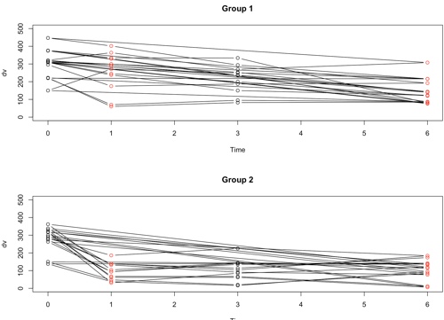
The following plots show the results of each individual subject broken down by groups. Earlier we saw the group means over time. Now we can see how each of the subjects stands relative to the means of his or her group. In the ideal world the lines would start out at the same point on the Y axis (i.e. have a common intercept) and move in parallel (i.e. have a common slope). That isn't quite what happens here, but whether those are chance variations or systematic ones is something that we will look at later. We can see in the Control group that a few subjects decline linearly over time and a few other subjects, especially those with lower scores decline at first and then increase during follow-up.
Plots (Group 1 = Control, Group 2 = Treatment)
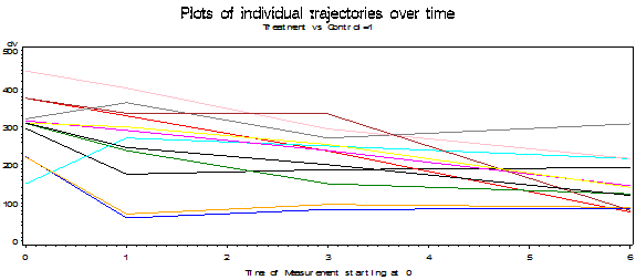

Toggle triangle to code and graphic using R
### I have no idea why the top line it each plot runs directly from Time0 to Time6.
### I have searched the code and find nothing wrong. But there are no
### such points in the data file.
par(mfrow = c(2,1))
Grp1 <- data2[Group == 1,]
plot(dv ~ time.cont, type = "b", data = Grp1, col = c(1:2), xlab = "Time",
 main = "Group 1", ylim = c(0,500))
Grp2 <- data2[Group == 2,]
plot(dv ~ time.cont, type = "b", data = Grp2, col = c(1:2), xlab = "Time",
 main = "Group 2", ylim = c(0,500))

_____________________________________________________________
As I said, I began with compound symmetry. But if you look at the actual correlations you will see that they come nowhere close to that. This means that we are going to have to do something to handle this problem. The actual correlations, averaged over the two groups using Fisher's transformation, are:
       Estimated R Correlation Matrix
     Row       Time1       Time2       Time3       Time4
       1      1.0000      0.5695      0.5351    -0.01683
       2      0.5695      1.0000      0.8612      0.4456
       3      0.5351      0.8612      1.0000      0.4202
       4    -0.01683      0.4456      0.4202      1.0000
In the printout above, there are also two other covariance parameters. Remember that there are two sources of random effects in this design. There is our normal σ2e, which reflects random noise. In addition we are treating our subjects as a random sample, and random variance among subjects is another source of variance that we need to contend with. This is written as E(MS) = σ2e + nσ2ρ. In the good old days when I was in graduate school, we used expected mean squares to justsify our choice of denominator for F ratios. That works with balanced designs, but starts to fall apart with unbalanced designs. Maximum likelihood works with both kinds of designs, which is one of its great strengths.
If you look at the SPSS data file that I load at WicksellLong.sav, you will see that there are two variables related to Time. One is called Time, and I later treat it as a factor with 4 levels. The other, labelled "Time.cont" records the month that the measurements were taken, namely 0, 3, 6, and 4.) If this were a standard ANOVA it wouldn't make any difference, and in fact it doesn't make any difference here, but when we come to looking at intercepts and slopes, it will be very important how we designated the 0 point. We could have centered time by subtracting the mean time from each entry, which would mean that the intercept is at the mean time. I have chosen to make 0 represent the pretest, which seems a logical place to find the intercept. The other times are indicated as 1, 3, and 6 months. I will say more about this later.
Missing Data
I have just spent considerable time discussing a balanced design where all of the data are available. Now I want to delete some of the data and redo the analysis. This is one of the areas where mixed designs have an important advantage. I am going to delete scores pretty much at random, except that I want to show a pattern of different observations over time. It is easiest to see what I have done if we look at data in the wide form, so the earlier table is presented below with '.' representing missing observations. (In my SPSS analyes I use "999" as the missing data value, and specify that when I load the data. R requires me to use "NA" as the missing value.) It is important to note that data are missing completely at random, not on the basis of other observations. The data file that I will read into SPSS will have the long format, and missing observations are simply indicated as 999, leaving us with 96 - 9 = 87 complete rows.
Group        Subj           Time0       Time1       Time3      Time6
1              1              296         175         187         192
1              2              376         329         236          76
1              3              309         238         150         123
1              4              222          60          82          85
1              5              150         999         250         216
1              6              316         291         238         144
1              7              321         364         270         308
1              8              447         402         999         216
1              9              220          70          95          87
1              10             375         335         334          79
1              11             310         300         253         999
1              12             310         245         200         120
2              13             282         186         225         134
2              14             317          31          85         120
2              15             362         104         999         999
2              16             338         132          91          77
2              17             263          94         141         142
2              18             138          38          16          95
2              19             329         999         999           6
2              20             292         139         104         999
2              21             275          94         135         137
2              22             150          48          20          85
2              23             319          68          67         999
2              24             300         138         114         174
If we treat this as a standard repeated measures analysis of variance, using the standard SPSS anova procedure, we have a problem. Of the 24 cases, only 17 of them have complete data. That means that our analysis will be based on only those 17 cases. Aside from a serious loss of power, there are other problems with this state of affairs. Suppose that I suspected that people who are less depressed are less likely to return for a follow-up session and thus have missing data. To build that into the example I could deliberately have deleted data from those who scored low on depression to begin with, though I kept their pretest scores. (I did not actually do this here.) Further suppose that people low in depression respond to treatment (or non-treatment) in different ways from those who are more depressed. By deleting whole cases I will have deleted low depression subjects and that will result in biased estimates of what we would have found if those original data points had not been missing. This is certainly not a desirable result.
To expand slightly on the previous paragraph, if we using Anova, we have to assume that data are missing completely at random, normally abbreviated MCAR. (See Howell, 2008.) If the data are not missing completely at random, then the results would be biased. But if I can find a way to keep as much data as possible, and if people with low pretest scores are missing at one or more measurement times, the pretest score will essentially serve as a covariate to predict missingness. This means that I only have to assume that data are missing at random (MAR) rather than MCAR. (I recognize that MAR is a very odd and confusing way to label data that are missing because of low initial scores, but that's the way we generally label such a design.) That is a gain worth having. MCAR is quite rare in experimental research, but MAR is much more common. Using a mixed model approach requires only that data are MAR and allows me to retain considerable degrees of freedom. (That argument has been challenged by Overall & Tonidandel (2007), but in this particular example the data actually are essentially MCAR. I will come back to this issue later.)
SPSS Anova results
The output from analyzing these data using SPSS Anova follows.(The Anova procedure uses casewise deletion by default.) I give these results just for purposes of comparison, and I have omitted much of the printout.
-----------------------------------------------------------------------------------------

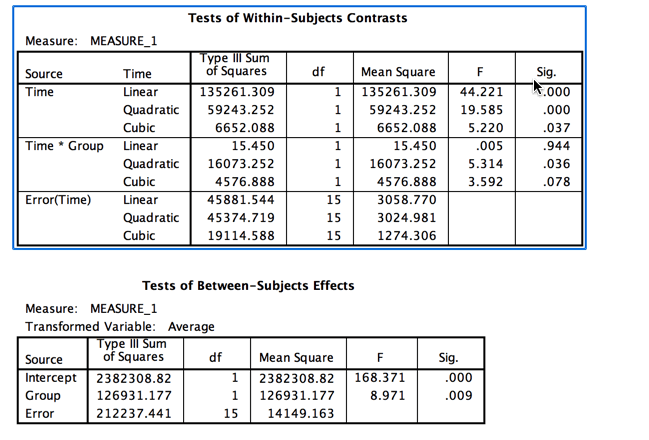
Notice that the output is split between Between-subjects terms and Within-subjects terms. We still have a group effect and a Time effect, but the F for our interaction has been reduced by about two thirds, and that is what we care most about. (In a previous version I made it drop to nonsignificant, but I relented here.) Also notice the big drop in degrees of freedom due to the fact that we now only have 17 subjects.
Mixed-Model
Now we move to the results using SPSS Mixed Models. I need to modify the data file by putting it in its long form and to replacing missing observations with 999, but that means that I just altered 9 lines out of 96 (10% of the data) instead of 7 out of 24 (29%). The syntax would look exactly the same as it did earlier. The results follow, again with much of the printout deleted. I requested that it use compound symmetry, but I will next move away from that.

What about R?
If you use R, as you will see later, you will not obtain exactly the same results for the main effects for at least two reasons. First of all, R defaults to Type I SS, whereas SPSS defaults to Type III. If you ask SPSS to use Type I, with the main effects in the same order, you come a bit closer, but not by much. As I have said elesewhere, R does not offer the same control over how it treats the covariance matrix, (and I don't know how it does it), so that may also explain part of the problem.
If you do run R using lmer (the important function in the lme4 package), you will have
### With random intercept
library(lme4)
Wick3 <- lmer(dv ~ Time*Group + (1|Subj), data = data3, contrasts = contr.sum)
anova(Wick3)
_______________________________________
Analysis of Variance Table
Df Sum Sq Mean Sq F value
Time        3 324543  108181 38.9502
Group       1  33334   33334 12.0018
Time:Group  3  73570   24523  8.8295
Notice that the interaction agrees with SPSS, but the other two Fs don't, in part because R is using Type I SS. But it is important to at least briefly mention the concept of "Random Intercept." In the code above, the part that says (1|Subj) specifies that each subject will be allowed his or her own intercept (that is what the "1" means). This helps to take care of those subjects who start off with low levels of depression, and those that start off with higher levels of depression. If we also wanted to allow each subject to have his or her own slope, we would use (1 +Time.cont|Subj), which would in part take recognition that subjects whon't all follow the same pattern of responses, and correlations will vary across the matrix. (Notice that I use the continuous (non-factor) version of Time.)
If we were using SAS, we would have an important addition to the printout. SAS would use the Wald chi-square to compare our model to the null model. This would give an overall test on whether this model fits better than a null model that does not include Group or Time. It is a chi-square test with chi-square = 19.21 and p = .0001. So it is a much better fit. The rest of the printout is a similar to an analysis of varinace on the fixed effects. This is a much nicer solution, not only because we have retained our significance levels, but because it is based on considerably more data and is not reliant on an assumption that the data are missing completely at random.
BUT Here is where things start to get interesting with maximum likelihood. There is a very strong argument to be made that we do not know the degrees of freedom for the denominator of the F and thus cannot calculate p exactly. This is not because statisticians are too dumb to work it out, but because it really is unknown. There are approximations and other ways of testing, which is why I mentioned the Wald test, but software such as R using lmer() won't even print out a column named p for fixed effects. [But try the lmerTest() library.] And that isn't all. This is where most treatments of mixed models veer off in a different direction, testing competing models instead of presenting a nice neat summary table.
Comparing models in R
The following will compare the models with and without varying slopes.
anova(model4, model5)
refitting model(s) with ML (instead of REML)
Data: data3
Models:
object: dv ~ Time * Group + (1 | Subject)
..1: dv ~ Time * Group + (1 + Time.cont | Subject)
       Df    AIC    BIC  logLik deviance  Chisq Chi Df Pr(>Chisq)
object 10 983.58 1008.2 -481.79   963.58
..1    12 978.91 1008.5 -477.45   954.91 8.6759      2    0.01306 *
---
Other Covariance Structures
To this point all of our analyses using SPSS have been based on an assumption of compound symmetry. (The assumption is really about sphericity, but the two are close and SPSS refers to the solution as type = cs.) But if you look at the correlation matrix given earlier it is quite clear that correlations further apart in time are distinctly lower than correlations close in time, which sounds like a reasonable result. Also if you looked at Mauchly's test of sphericity (not shown) it is significant with p = .012. While this is not a great test, it should give us pause. We really ought to do something about sphericity.
One thing that we could do about sphericity is to specify that the model will make no assumptions whatsoever about the form of the covariance matrix. To do this in SAS or SPSS I will ask for an unstructured matrix. This is accomplished by using the dropdown menu to select Unstructured or, in SAS, by including type = un in the repeated statement. This will force the program to estimate all of the variances and covariances and use them in its solution. The problem with this is that there are 10 things to be estimated and therefore we will lose degrees of freedom for our tests. But I will go ahead anyway. For this analysis I will continue to use the data set with missing data, though I could have used the complete data had I wished. The results are shown below using SPSS for the analyses.
Results Using Unstructured Matrix

Notice the matrix of covariances. They are all over the place, ranging from 5163.816 to -129.831. That certainly doesn't inspire confidence in compound symmetry.
The Fs have not changed very much from the previous model, but the degrees of freedom for within-subject terms have dropped from 57 to 22, which is a huge drop. That results from the fact that the model had to make additional estimates of covariances.
But we have gone from one extreme to another. We estimated two covariance parameters when we used type = cs and 10 covariance parameters when we used type = un. (Put another way, with the unstructured solution we threw up our hands and said to the program "You figure it out! We don't know what's going on.' There is a middle ground (in fact there are many). We probably do know at least something about what those correlations should look like. Often we would expect correlations to decrease as the trials in question are further removed from each other. They might not decrease as fast as our data suggest, but they should probably decrease. An autoregressive model, which we will see next, assumes that correlations between any two times depend on both the correlation at the previous time and an error component. To put that differently, your score at time 3 depends on your score at time 2 and error. (This is a first order autoregression model. A second order model would have a score depend on the two previous times plus error.) In effect an AR(1) model assumes that if the correlation between Time 1 and Time 2 is .51, then the correlation between Time 1 and Time 3 has an expected value of .5122 = .26 and between Time 1 and Time 4 has an expected value of .5133 = .13. Our data look somewhat close to that. (Remember that these are expected values of r, not the actual obtained correlations.) The solution using a first order autoregressive model follows.
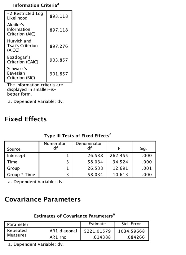
Now we have three solutions, but which should we choose? One aid in choosing is to look at the "Fit Statistics' that are printed out with each solution. (I did not show these statistics for the first two analyses, but they are there for the Autoregressive solution.) These statistics take into account both how well the model fits the data and how many estimates it took to get there. Put loosely, we would probably be happier with a pretty good fit based on few parameter estimates than with a slightly better fit based on many parameter estimates. If you look at the three models we have fit for the unbalanced design you will see that the AIC criterion for the type = cs model was 909.4, which dropped to 903.7 when we relaxed the assumption of compound symmetry. A smaller AIC value is better, so we should prefer the second model. Then when we aimed for a middle ground, by specifying the pattern or correlations but not making SAS estimate 10 separate correlations, AIC dropped again to 897.1. That model fit better, and the fact that it did so by only estimating a variance and one correlation leads us to prefer that model.
Where do we go now?
There is a lot that has been written about mixed models, and not all of it is very clear. The best introduction that I know is a page by Bodo Winter. He does an excellent job of working through the logic without overwhelming the reader with equations or code. The basic code that he uses is R, but you can benefit from his page even if you don't use R. The link is http://www.bodowinter.com/tutorial/bw_LME_tutorial2.pdf.
This document is sufficiently long that I am going to create a new one to handle this next question. In that document we will look at other ways of doing much the same thing. The reason why I move to alternative models, even though they do the same thing, is that the logic of those models will make it easier for you to move to what are often called single-case designs or multiple baseline designs when we have finished with what is much like a traditional analysis of variance approach to what we often think of as traditional analysis of variance designs.
For the second part go to Mixed-Models-for-Repeated-Measures2.html
References
Guerin, L., and W.W. Stroup. 2000. A simulation study to evaluate PROC MIXED analysis of repeated measures data. p. 170-203. In Proc. 12th Kansas State Univ. Conf. on Applied Statistics in Agriculture. Kansas State Univ., Manhattan.
Howell, D.C. (2008) The analysis of variance. In Osborne, J. I., Best practices in Quantitative Methods. Sage.
Little, R. C., Milliken, G. A., Stroup, W. W., Wolfinger, R. D., & Schabenberger, O. (2006). SAS for Mixed Models. Cary. NC. SAS Institute Inc.
Maxwell, S. E. & Delaney, H. D. (2004) Designing Experiments and Analyzing Data: A Model Comparison Approach, 2nd edition. Belmont, CA. Wadsworth.
Overall, J. E., Ahn, C., Shivakumar, C., & Kalburgi, Y. (1999). Problematic formulations of SAS Proc.Mixed models for repeated measurements. Journal of Biopharmaceutical Statistics, 9, 189-216.
Overall, J. E. & Tonindandel, S. (2002) Measuring change in controlled longitudinal studies. British Journal of Mathematical and Statistical Psychology, 55, 109-124.
Overall, J. E. & Tonindandel, S. (2007) Analysis of data from a controlled repeated measurements design with baseline-dependent dropouts. Methodology, 3, 58-66.
Pinheiro, J. C. & Bates, D. M. (2000). Mixed-effects Models in S and S-Plus. Springer.
Some good references on the web are:
http://www.ats.ucla.edu/stat/sas/faq/anovmix1.htm
http://www.ats.ucla.edu/stat/sas/library/mixedglm.pdf
The following is a good reference for people with questions about using SAS in general.
http://ssc.utexas.edu/consulting/answers/sas/sas94.html
Downloadable Papers on Multilevel Models
Good coverage of alternative covariance structures
http://cda.morris.umn.edu/~anderson/math4601/gopher/SAS/longdata/structures.pdf
The main reference for SAS Proc Mixed is
Little, R.C., Milliken, G.A., Stroup, W.W., Wolfinger, R.D., & Schabenberger, O. (2006) SAS for mixed models, Cary, NC SAS Institute Inc.
See also
Maxwell, S. E. & Delaney, H. D. (2004). Designing Experiments and Analyzing Data (2nd edition). Lawrence Erlbaum Associates.
The classic reference for R, though it is based on an older library, is Penheiro, J. C. & Bates, D. M. (2000) Mixed-effects models in S and S-Plus. New York: Springer.

Last revised 4/10/2016