

This web page is a step by step demonstration of using NORM (give ref.) to handle multiple imputation. It is deliberately not a theoretical discussion. You can download the Windows version of NORM from http://www.uvm.edu/StatPages/Missing_Data/NormProgram.zip. That is not a very new program, but it works nicely and until they revise it, it is what we have. There is also a version that runs under R for those who are comfortable with R.
Because I used NORM to analyze the data file on behavior problems of children with of cancer patients in what I have called Part 2 of the missing data page, I will use a different data file here. The data file is named GuberNoHead999.dat and contains variables related to educational achievement and expenditures. This is a data file from a study by Guber ((1999) which I discuss in both of my texts. The goal of the analysis will be to look at academic performace as measured by a state's mean SAT score. (ETS strongly argues against using SAT scores in this way, and the analysis will show one reason for their concern.) The independent variables are the mean state Expenditure for secondary education, the mean pupil/teacher ratio (PTratio), the mean salary (Salary), the mean verbal test score (Verbal), the combined math and verbal SAT score (SAT), and the logarithm of the percentage of students in each state taking the SAT. The natural log was used to help improve the distributiom of that variable. I also included in the file the states' mean ACT score and the percentage of students taking the ACT, though I did not include these in the final analysis. It is important to note what variables I did NOT use. I had the Math SAT score and the PctSAT included, but immediately ran into trouble. The SAT is simply the sum of the Verbal and Math scores, and the LnPctSAT is simply the log of the PctSAT. If I left those in, the solution would fail with the notation that the matrix is not positive definite. What this means is that there is a perfect correlation between some of the variables. I left those variables out to get around this problem. I also left the state name out because NORM does not like string variables.
The data file has missing observations, which are denoted by "999." These were not missing in Guber's data--I just randomly eliminated values to create an example. It turns out that the results that I will come up with are close to what I obtain using her complete data.
The first few cases are shown below. I have given the variable names on the first line, but they would not be included in the file that NORM sees. NORM won't support that. Missing data are indicated by 999. NORM only allows a few codes for missing, and 999 is one of them, but "." is not.
ID	Expend	PTratio	Salary	Verbal	SAT	PctACT	ACT	LnPctSAT
1	4.405	17.2	31.144	491	1029	61	20.2	999
2	8.963	17.6	47.951	445	934	32	21	3.85
3	4.778	19.3	32.175	448	944	27	21.1	3.296
4	999	17.1	28.934	482	1005	66	20.3	1.792
5	4.992	24	41.078	417	902	11	21	3.807
6	5.443	18.4	34.571	462	980	62	21.5	3.367
7	8.817	14.4	999	431	908	3	21.7	4.394
8	7.03	16.6	39.076	429	897	3	21	4.22
9	5.718	19.1	32.588	420	889	36	20.7	3.871
10	5.193	16.3	32.291	406	854	16	20.2	4.174
11	6.078	17.9	38.518	407	889	17	21.6	999
12	4.21	19.1	29.783	468	979	62	21.4	2.708
To enter the data start NORM.exe and select File/New Session. Then select the file, which I called GuberNoHead999.dat, reflecting the fact that I have removed the variable names in the header line and have used "999" for missing.
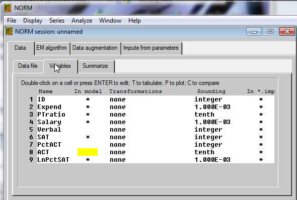
The Help files in NORM are excellent (mostly). The first screen that we see after we start a new session and read in the data is shown below. On that screen you can see that I have filled in the variable names. To the right you see a column of asterisks. By double clicking on one of those you can remeove that variable from the imputation procedure. If you go back to the menu tagged as "Data file" you will be able to tell it that "999" is the missing value. If you go to Summarize, you can print out information on which variables have missing data and how many observations are missing. The percentage of missing values ranged from 0% to 10% for the individual variables, buit if we were to use listwise deletion we would throw away 12 cases, which is 24% of our data.
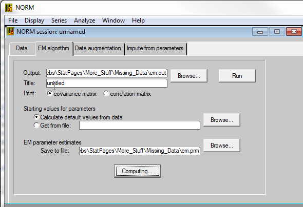
The next step that you want to carry out is to run the EM algorith. This estimates means, variances, and covariances in the data. First a bit of theory. EM looks at the data and comes up with estimates of means, variances, and covariances. Then it uses those values to estimate missing values. But when we add in those missing values, we come up with new estimates of means, variances, and covariances. So we again estimate missing values based on those estimates. This, in turn, changes our data and thus our next estimates. But for a reasonably sized sample, this process will eventually converge on a stable set of estimates. We stop at that point. The screen for that procedure is shown below. You don't really have to do anything on this screen except run it if you are willing to take the defaults. We run EM first before we go on to Data augmentation to get a reasonable set of parameter estimates to use in the next step. We don't have to do this first, but it speeds the process. You simply select the EM algorithm tab, give the output file a name (the default is em.out) You can specify the maximum number of iterations. If it does not converge by then, it will quit. The default is 1000. The parameter estimates that result from the EM algorithm are stored, by default, in a file named em.prm. I won't change this because then I would have to make the same change in subsequent steps that use this file. It's easier to go along with the defaults. Just click Run The results will appear. There are actually two files--one is for you to read and the other (em.prm) is for NORM to use later.
Next you want Data Augmentation. Data Augmentation (DA) is the process that does most of the work for you. It takes estimates of population means, variances, and covariances, either by taking the output of EM or by recreating them itself. Again we need a tiny bit of theory. Using the means, variances, and covariances, DA first estimates missing data. But then it uses a Baysian approach to create a likely distribution of the parameter values. For example, if the mean with the adjusted data comes out to be 52, it is reasonable to expect that the population mean falls somewhere around 52. But instead of declaring it to be 52, DA draws an estimate at random from the likely distribution of means. This is a Baysian estimate because we essentially ask what would the distribution of possible means really look like given the obtained sample mean. To oversimplify, think of calculating a sample mean on the basis of data. Then think of creating a confidence limit on the population mean given that sample mean. Suppose that the CI is 48 - 56. Then think of randomly drawing an estimate of mu from the interval 48-56, and then continuing with an iterative process. This is greatly oversimplified, but it does contain the basic idea. And, remember, we are going to continue this process until it converges.
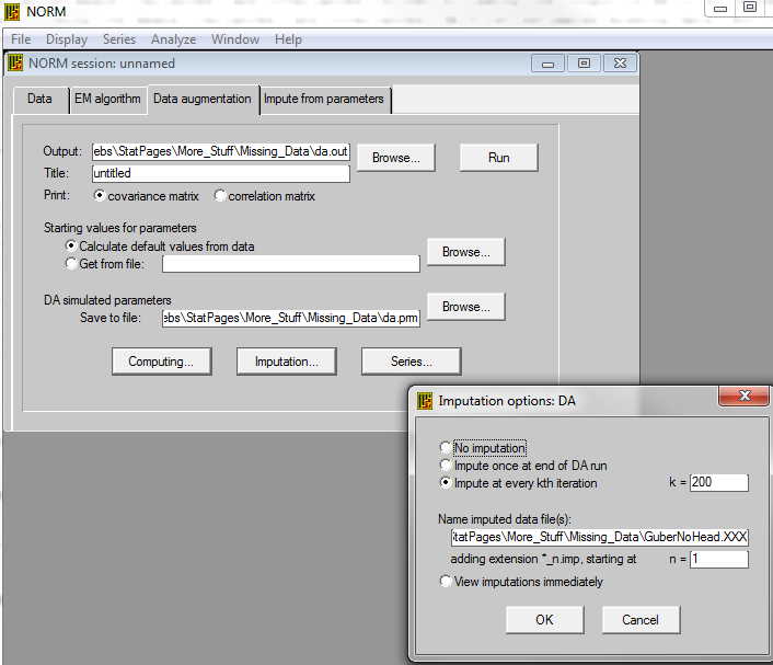
To run DA, you could take the defaults by clicking on the Data Augmentation tab. However, we need to do a little more because we want to create several possible sets of data. In other words, we want to run DA and generate a set of data. Then we want to run DA over again and create another set. In all we might create 5 sets of data, each of which is a reasonable sample of complete data with missing values replaced by estimated values.
Rather than run the whole program 5 times, what we do is to run it, for example, through 1000 iterations. In other words, we will go through the process 1000 times, each time estimating data, then estimating parameters, then re-estimating data, etc. But after we have done it 200 times, we will write out that data set and then keep going. After 200 iterations we will write out another data set, and keep going. After the 1000th iteration we will write out the 5th data set. You can see the relevant windows below. We use the "Computing button to tell it to run 1000 iterations. Then we use the "Imputation button to tell it to write out every 200th interation, giving us five sets of output in all. (When you enter the "200," be sure to click the button to its left.)
Now you have 5 complete sets of data, each of which is a pretty good guess at what the complete data would look like if we had it. We would HOPE that whichever data set we used we would come to roughly the same statistical conclusions. For example, if our analysis were multiple regression, we would hope, and expect, that each set would give us pretty much the same regression equation. And if that is true, it is probably reasonable to guess that the average of those five regression equations would be even better. For example, we would average the five estimates of the intercepts, the five estimates of b1, etc. We won't do exactly this, but it is close.
But you might ask why I chose 1000, 200, and 5. Well, the 5 replications was chosen because Rubin (1987) said that 3 - 5 seemed like a nice number. Well, it was a bit more sophisticated than that, but I'm not going there. So let m = 5. But how many interations before we print out the first set of imputed data? Schafer and Olsen (1989) suggest that a good starting point is a number larger than the number of iterations that EM took to converge, which, for our data, was 56. So I could have used 60, but k = 200 seemed nice. Actually it was overkill, but that won't hurt anything, and you are not going to fall asleep waiting for the process to go on for k*m = 1000 times. It will take a couple of seconds.
This is the point at which we put NORM aside for the moment and pull out SPSS or something similar. We simply take our m = 5 datasets, read them each into SPSS, run our 5 multiple regressions, record the necessary information, and turn off SPSS. For this example I chose to predict SAT from Expend, PTratio, and LnPctSAT. (Notice that I included all 8 variables when I did the imputations because even variables that I might not use in my analysis may contribute something to estimating missing values. For example, a state's mean Salary may help predict a Expend score. (The correlation is .85.)
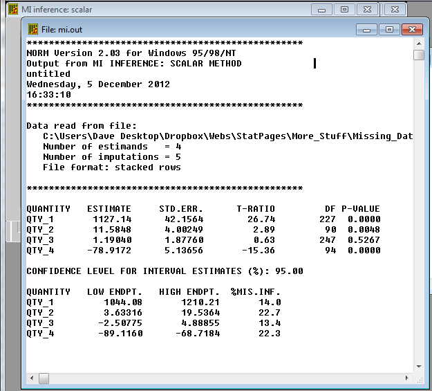
I suggested above that you are basically just going to average the coefficients from the 5 regressions--or similar stuff from 5 analyses of variance, logistic regressions, chi-square contingency table analyses, or whatever. Well, that is sort of true. In fact for the actual coefficients that is exactly true. But we also want to take variability into account. Whenever you run a single multiple regression you know that you have a standard error associated with each bi. Square that to get a variance. But you also know that from one of the 5 analyses to another you are also going to have variability. We want to combine the within-analysis variance and the between-analysis variance and use that to test the significance of our mean coefficient. I show below how to do this by hand, but you can use NORM to do it if you want. Just make up the file shown below (the 10 lines of estimates), call it something like CombinedResults.dat, and go to the tag for "Analyze/MI Inference: Scalar", change the number of estimands to 4 (3 predictors plus the intercept), and run the program. Those results appear below.
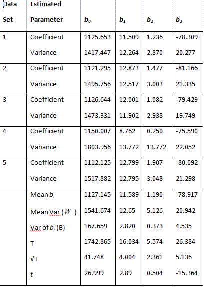
The table that follows contains the results of the 5 imputations. I have included it simply to illustrate the computations by hand, but, with one minor exception, it agrees completely with the table above.
Thus the regression equation for the first set of data would be
Y = 1125.653 + 11.509*Expend + 1.236*PTratio -78.309*LnPctSAT.
Now we proceed in several steps, the results of which you can see near the bottom of the table.
- Calculate the mean value (over the five imputations) for each of the regression coefficients and record those.
- Calculate the means of the squared standard errors for each coefficient (the even-numbered line of the table), and record those.
- Calculate the variance of the five bi for each variable and the intercept.
The four coefficient means that I calculated in the first step are the best estimates of the corresponding parameters. (I should point out that if you are using NORM to do this set of calculations, you want to enter the standard error, the square root of the variance, rather than the variance. I took me forever to figure out what I had done wrong!) Thus the best
equation for this prediction is
Ŷ = 1127.145 + 11.589*Expend + 1.190*PTratio - 78.917*LnPctSAT
Now we need to calculate the standard error of each coefficient. To do that we will combine the variances of each coefficient in each imputation plus the variances of each coefficient across the 5 imputations. The formula for doing this is
T = mean variance within () + (1 + 1/m)*variance (B) of the bi.
which is
T = W̄ + (1 + 1/m)*B
For b1 this is 2.692 + (1+1/5)*4.859 = 8.523.
The square root of this is 2.919, which is our estimate of the standard error of the estimated b1 = -4.000. If we divide -4.000 by 2.919 we get -1.370, which is a t statistic on that coefficient. So that variable does not contribute significantly to the regression.
You will note that I used multiple regression here. If I had used an analysis of variance on these data I would have run 5 Anovas and done similar averaging. I haven't really thought through what that would come out to, but it shouldn't be too difficult. I suspect that I would average the MSbetween, average the MSwithin, take the variance of the SSbetween, and combine as I did above. I can work this out a bit better when I get SAS going--again.
I have shown how to do this with NORM. As I have said elsewhere, you can also do something similar with SPSS and with SAS. (I am repeating myself for those who have not worked their way through previous pages.) In addition, you can run NORM from within R. The code for doing that is available at Norm.R. There is an R program called Amelia (in honor of Amelia Earhart). I have written (or will write) instructions for the use of that program. An important point, however, is that each program uses its own algorithm for imputing data, and it is not always clear exactly what algorithm they are using. For all practical purposes it probably doesn't matter, but I would like to know.
- For a page on SPSS, go to MissingDataSPSS.html.
- For SAS, see MissingDataSAS.html.
- For Amelia (when I (ever) write it) see MissingDataAmelia.html.
Last revised 6/29/2015