Logistic Regression With Missing Data

David C. Howell

Missing data are a part of almost all research, and we all have to decide how to deal with it from time to time. I have written two web pages on multiple regression with missing data. You can see these at (Missing-Part-One.html and Missing-Part-Two). That first page covers the basic issues in the treatment of missing data, so I will not go over that ground here. Instead I will focus on the process of "imputing" observations to replace missing one when using logistic regression. The process is not a lot different, but it gives me a chance to use another data set that provides a convenient reference point because it started out with complete data.

Logistic regression is very similar to a standard multiple regression where the dependent variable is a dichotomy. In fact, if the outcome proportions are no more extreme than about .20/.80, the results obtained from both will be fairly similar.

I am going to use a set of data from a study that I was involved with some time ago and published as Epping-Jordan, Compas, & Howell (1994). It dealt with cancer outcomes (improved versus not improved) as a function of several variables. These include Survrate (a rating by the oncologist of the individual's expected survival time, Prognosis (a four point scale), Amttreat (amount of treatment), GSI (the Global Symptom Index from Derogatis' Symptom Checklist 90), Avoid (a measure of avoidance behavior), and Intrus (a measure of intrusive thoughts). The original data are available at survrate.dat. For this example I doubled the sample size by randomly adding or subtracting random numbers to or from the data in the original set. This left me with the original 66 cases and an additional 66 pseudocases. I did this simply to create a better example. The full set of 132 cases had no missing observations. so we can begin with a logistic regression on a full data set and use these results for comparison with what we find with missing data. The first few lines of this data set is shown below.

count id outcome survrate prognos amttreat gsi avoid intrus
1 105 1 33 3 2 0.35 17 20
2 106 1 50 2 3 0.375 7 15
3 107 1 91 3 2 0.275 15 7
4 108 1 90 3 2 0.2 2 2
5 109 1 70 3 3 0.375 23 27
6 111 2 31 2 2 0 19 10
7 112 1 91 2 3 0.175 6 16
8 113 1 81 3 2 0 3 9
9 114 2 15 1 2 0.125 19 13
10 116 2 1 1 2 0.875 15 7

Analysis Using SAS

The SAS code for this analysis follows. Notice that only four predictors are used for the analysis, and one of those might best be dropped.

Data Data;
	Infile 'https:www.uvm.edu/~dhowell/StatPages/Missing_Data/Missing-Logistic/survDoubledNM.dat';   /* Complete data  */
	Input count id outcome01 survrate prognos amttreat gsi avoid intrus;
run;

Proc Logistic data = Data;   /* Logistic regression with 4 predictors */
     class  outcome01;
	 model  outcome01 = survrate gsi avoid intrus  /covb;
	 ods output ParameterEstimates = lgsparms  CovB = lgscovb;
run;

Notice several things. Near the top of the printout we have a Likelihood Ratio test on the null hypothesis that there is no relationship between these predictors and the dependent variable. That is certainly significant. That test is roughly equivalent to the overall F test for a multiple correlation coefficient. Above those statistics are three fit statistics that we use to test reduced models. For example, we might use those statistics to see if there is a significant drop in predictability if we were to drop Intrus as a predictor. We may come to that later. Notice that if you take -2 Log Likelihood for a model with no predictors and one with four predictors, you get 154.691 - 57.243 = 97.448, which is the log likelihood that we just used to test the overall model.

Next in the printout we come to the Analysis of Maximum Likelihood Estimates. These are analgous to the standard regression coefficients and their tests in multiple regression, although these are chi-square tests instead of t tests. The intercept and the coefficients for survrate, gsi, and avoid are all significant, but the test on intrus is not. We rarely care about the intercept, but the others are important.

Moving to Missing Data

Having a full data set, I randomly deleted 35 observations and replaced them with a missing data code. Because this truly was a random process, the data are missing completely at random (MCAR). This file for SAS is available at survrateMissingDOTNH.dat. The DOT in that title indicates that for this particular set I used "." as a missing data code. (For SPSS I will change "." to "999", and for R I will change "." to "NA." For some software I will include variable labels in line 1, and for other software I will leave the labels out. The "NH" indicates that there is not a header for this file.)

Analysis with Missing Data

Before we go ahead and impute data for the missing values, we will look at an analysis that is based on the file that contains missing data. The SAS commands would be the same as those that we just used, except that we would first read in the file with missing data and use that for the analysis. The results of that analysis follow.

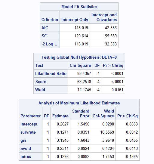
The results of this analysis are quite similar even though we have eliminated 35 observations. The test on the intercept is no where near significant, but the other tests are similar to what they were with missing data. Again intrus is not a significant predictor. It is my experience, and it may just be my imagination, that tests on the intercept, and, indeed, the value of the intercept itself, seem to be all over the place. Since we rarely care about the intercept anyway, I am not going to get too excited about this.

Replacing Missing Data With Imputed Values

Rather than simply putting up with the fact that data are missing, we are probably in better shape if we make intelligent guesses as to what those missing values would have been if we had been able to collect them, and then go ahead by including those "guesses" in our data. There is a significant literature on this topic, and I discuss parts of it in other web pages, including the ones given at the beginning of this page (especially the second one). I will not repeat that discussion here, but will move directly to the process known as multiple imputation (MI). I will use several different software packages for this purpose, partly because I want to discuss how to use those packages and partly to compare the results that we obtain.

Multiple Imputation

There are a number of alternative ways of dealing with missing data, and this document is an attempt to outline those approaches. The original version of this document spent considerable space on using dummy variables to code for missing observations. That idea was popularized in the behavioral sciences by Cohen and Cohen (1983). However, that approach does not produce unbiased parameter estimates (Jones, 1996), and is no longer to be recommended--especially in light of the availability of excellent software to handle other approaches. For a very thorough book-length treatment of the issue of missing data, I recommend Little and Rubin (1987) .A shorter treatment can be found in Allison (2002) . Perhaps the nicest treatment of modern approaches can be found in Baraldi & Enders (2010), a modified version of which can be found at Baraldi & Enders. I have also written a chapter on missing data for an edited volume (Howell, 2007). Part of that paper forms the basis for some of what is found here, and is available at Missing Data Paper .

As I said, mutiple imputation is concerned with replacing missing observations with reasonable estimates and then proceeding from there. But the word "multiple" does not refer to multiple variables, but with generating multiple data sets using imputation, analyzing each data set, and then averaging the results over those analyses. The printout that will follow comes from using Proc MI and Proc MIAnalyze in SAS. We will soon see solutions using other software.

The SAS command for the imputation process is quite simple. The code is:

Proc MI Data = Missing out = miout nimpute = 5 seed = 35399;  /*Impute using all predictors */
	Var outcome01 survrate prognos amttreat gsi avoid intrus;

For this procedure we first specify the missing data, which I named Missing when I read them in. I then specify an output data set with imputed values. The output is an internal "data set," not a data file. It won't write to a file but it will create an internal data set that the next procedures will use. The command "nimpute = 5" sets the number of imputed data sets that will be created. Five is a common value for nimpute. Finally I specify a random seed. If I leave this out, SAS will pick one, but it will pick a different one each time I run the program. I want to be sure that if I go back and redo that analysis for some reason, it starts at the same point in a sequence of random balues, which is why I bother to specify it.

The second line of syntax specifies the variables to be used in the imputation. I have specified that it should use all of the variables, except the trivial one of ID. I will NOT be using all of these variables in my final analysis, but I include them here for what they are able to contribute to finding suitably pseudovalues. For example, I don't care very much for the AmtTreat variable, but it might help explain part of the variance in Outcome01, and I include it for that reason.

When this program runs it will produce a large new dataset with 5 * 132 = 660 cases. It will also include a variable called Imputation. The first 132 cases will have Imputation = 1, the next 132 have Imputation = 2, and so on. The reason for this is that we will later perform an analysis on each set of imputed data separately.

I don't show the results of this analysis, again using SAS, but rest assured that it has created five complete data sets piled one on top of another. There is a slight problem with these data sets in that missing values of Outcome01 have been replaced with non-integer numbers. The replacement values should be 0 or 1, because those are the only legitimate values for Outcome01. So the following bit of code corrects that problem by rounding the decimal values up or down to 0 or 1. The code for this is:

data cleaned;
    set miout;
	if outcome01 < .50 then outcome01 = 0;
	if outcome01 >= .50 then outcome01 = 1;
run;

The new data set is named "cleaned," and that is what we will use for the next analysis.

Now that we have five data sets with complete data and with Outcome01 coded correctly as 0/1, we will run five separate logistic regressions, saving the results of each. Thus for each run we will have, among other things, regression coefficients and their standard errors for each variable. We need these because the last set of code will effectively average these results. The code for the regression is :

Proc Logistic data = cleaned outest=outreg covout;   /* Logistic regression on imputed 
                                             		    files separately */
     class  outcome01;
	 model  outcome01 = survrate prognos amttreat gsi avoid intrus ;
	 by _Imputation_;
	 ods output ParameterEstimates = lgsparms  CovB = lgscovb;
run;

Notice that we have specified that the new data file is named "cleaned." and that the outcomes of this procedure are to be stored in a data set named "outreg." Notice also that we specify that Outcome01 is a class variable, meaning that it has, in this case, two possible values. The model statement is similar to the one we used earlier, but notice the important addition of "by _Imputation_;" This returns a separate analysis for each set of data.

Now we are ready to perform the final analysis, which takes the results of the five logistic regressions and combines them. The code for this analysis follows:

proc MIANALYZE data = outreg;   /* Read in parameter estimates and pool */
	Var   intercept survrate gsi avoid intrus;
run;

There is something slightly different about the code for this procedure. All along we have had a variable named outcome01, but the logistic regressions will not produce a coefficient named that. Instead it returns coefficients named "intercept","Survrate", etc. So we need to use the term "intercept" in this analysis. The results follow:

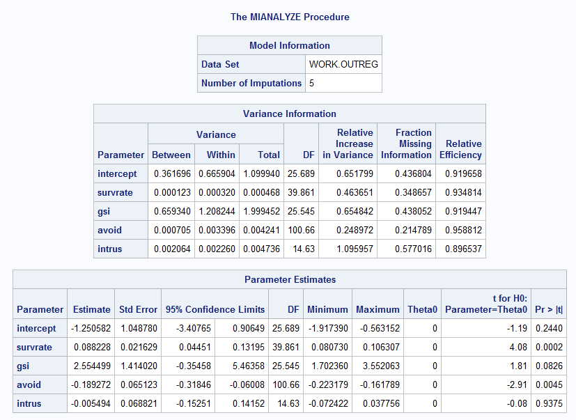
In the web page referred to at the beginning of this page I show how to combine across imputed estimates. I won't repeat that here, but basically we average across the five sets of coefficients, we average across the standard errors, and we take the variability of regression coefficients across the five sets of imputed data. You can see the results of doing that in the printout. What is most important is the last table. It gives the overall coefficients for the intercept and predictors and provides a test of significance for each. Thus our final logistic regression equation is

Ŷ = -1.251 + 0.088 * survrate + 2.555 * gsi - 0.189 * avoid - 0.005 * intrus

Here survrate and avoid are significant, but intrus certainly is not. These results can be compared against the original complete data set. There clearly are differences, but the same general pattern of results emerges. Survrate and avoid are significant predictors, gsi is nearly significant, and intrus is clearly not significant. If I were writing up these data I would rerun the analyses without intrus.

Now to SPSS

We can perform the same basic analyses using SPSS. I am not going to repeat everything, but I will repeat some things. In the first place, I will run the analysis using the file with missing data. Because these are exactly the same data that were used is SAS, we should obtain the same results. The difference will come mainly in the components that SPSS prefers to print out. The code for this analysis is:

DATASET ACTIVATE DataSet1.
LOGISTIC REGRESSION VARIABLES outcome01
  /METHOD=ENTER survrate gsi avoid intrus 
  /CLASSPLOT
  /PRINT=GOODFIT
  /CRITERIA=PIN(0.05) POUT(0.10) ITERATE(20) CUT(0.5).

Notice that I am still using four predictors and that outcome01 is the dependent variable. The results of this analysis follow:

This printout is the same as the one from SAS in terms of the regression coefficients. From that table you see that the significance test on the regression produces the same -2LogLikelihood as we had before. From the table at the bottom you can see that the regression coefficients are the same, and you can also see a table of classifications. From the first row you can see that out of 72 cases that really had a classification of 0, 6 of those were incorrectly classified as 1. Four out of 27 outcomes that were really a 1 were misclassified as 0. Thus 10/132 = 8% were misclassified, but 92% were correctly classified. That is encouraging.

Multiple Imputation Using SPSS

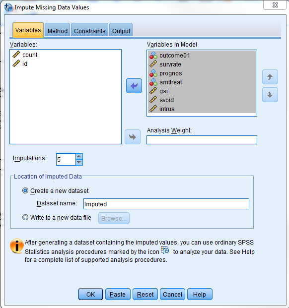
To do multiple imputation in SPSS you go to Analyze/Multiple Imputation/Impute missing data values. Here you specify all of the variables that we will use for that procedure, which will be the same ones that we used with SAS. Notice that we don't distinquish between independent and dependent values. The GUI screen and the SPSS syntax follow.

*Impute Missing Data Values.
DATASET DECLARE Imputed.
MULTIPLE IMPUTATION outcome01 survrate prognos amttreat gsi avoid intrus 
  /IMPUTE METHOD=AUTO NIMPUTATIONS=5 MAXPCTMISSING=NONE 
  /MISSINGSUMMARIES NONE 
  /IMPUTATIONSUMMARIES MODELS 
  /OUTFILE IMPUTATIONS=Imputed .

You will notice that I have specified 5 imputation data sets and I have declared the name of the internal data set to be "Imputed". The Imputed data set will have five sets of 132 records each, and my next analysis will analyze those data sets separately and then combine the results in a way that is similar to what we did with SAS. (Actually that file with have 6 data sets because the original 132 cases will appear as Imputation #0 and will be ignored in the next analysis.

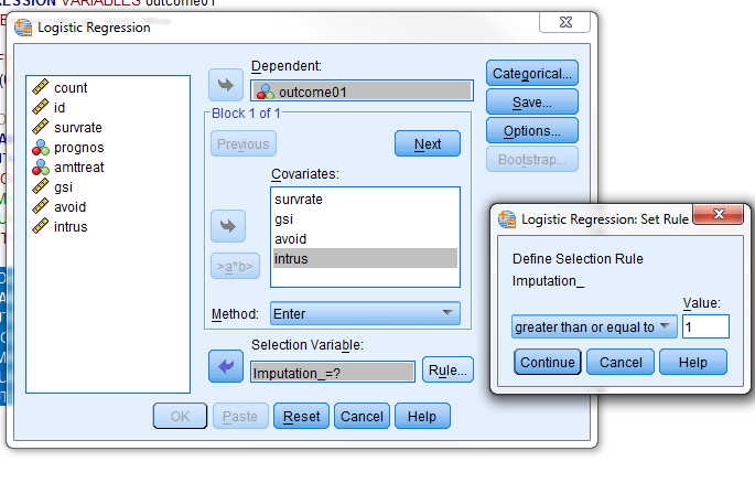
Now that we have the imputed data set, we can run the analysis on that. SPSS works a little differently from SAS. If you use the dropdown menus to call up Regression, you will see several choices. Some of them have something that looks like a snail with dots behind it. You may use any of those. We will choose binary logistic regression. The following window will appear. To get the smaller window labeled "Logistic Regression Set Rule," just click on the "rule" link just above "help."

DATASET ACTIVATE Imputed.
LOGISTIC REGRESSION VARIABLES outcome01
  /SELECT=Imputation_ GE 1
  /METHOD=ENTER survrate gsi avoid intrus 
  /CRITERIA=PIN(.05) POUT(.10) ITERATE(20) CUT(.5).

The printout from SPSS is not as pretty as with SAS, but the information that you need is there. SPSS shows the logistic regressions for each imputation, and then combines them at the bottom. These are the results that we are most interested in.

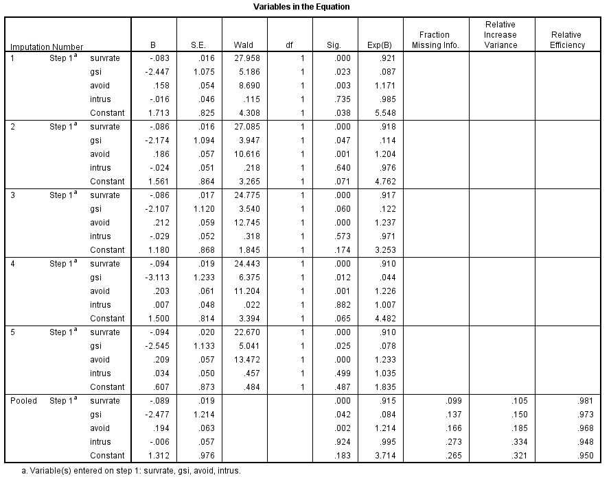
From this analysis our regression equation is

Ŷ = 1.312 - 0.089 * survrate - 2.477 * gsi + 0.194 * avoid - 0.006 * intrus

Compare this with the result that we found with SAS, which follows.

Ŷ = -1.251 + 0.088 * survrate + 2.555 * gsi - 0.189 * avoid - 0.005 * intrus

Notice that there is remarkable agreement on the coefficients with one notable difference. The SAS coefficients are of the opposite sign from the SPSS coefficients. This is really not a meaningful difference. It stems from the fact that one program is trying to predict the outcome coded as 0 and the other is trying to predict the outcome coded as 1. One is just the reverse of the other.

Now to NORM

Schafer (1997, 2000) has written a program called NORM and a set of functions in R, also called norm. We will start with the stand-alone program (norm.exe), it was available at http://sites.stat.psu.edu/~jls/norm203.exe, but Schafer moved from there some time ago. You can, however, find a copy at Missing_Data/NormProgram.zip I will cover this analysis quickly, because the page is getting awfully long. You begin by downloading the file and opening norm.exe.

The opening screen is shown below. There are two things to keep in mind. norm.exe does not like to have variable names in the first line, so delete them and enter them after the data have been loaded. In addition, you can not use NA to indicate missing data as you do in the R version. So I used 999.

You first need to start norm.exe, by clicking on its icon, and then specify that you want a new session. Find the data file and enter it. The first screen that will come up once the data have been loaded looks like:

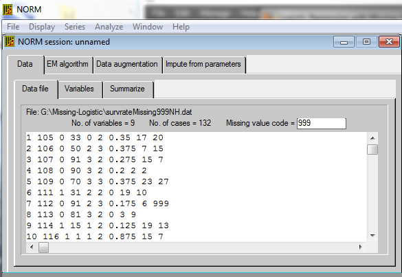
On this screen you can specify that 999 is the coding for missing data. Check to see that the data look reasonable, and then click on the "variable" tab, where you will name your variables. That screen looks like:

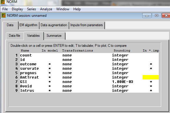
Your first column will look different until you change the variable names. Notice that there is a column labeled "In Model." There should be an asterisk next to each variable that you want to be part of the final model. In my case this is outcome, survrate, gsi, avoid, and intrus. Just click on the asterisks that you don't want and they will go away. Then go on to the Summarize tab, specify an output file, and click run. That will show you the pattern of missing data and the basic descriptive statistics. You can ignore this step if you wish, but it is a good way to catch errors.

The next step is to run the EM algorithm. This will give us good starting points from which to begin our imputations. I think that it makes sense to take the default file names. If you click on the Computing button you can specify the maximum number of iterations that we be allowed before the program throws up its hands and says "This is never going to settle down to a reasonable set of answers." The default of 1000 is probably more than enough. If it won't settle down by then, check to see if one of your variables is a perfect combination of other variables. For example, I recently had a problem with data that had an SAT verbal score, and SAT math score, and an SAT total score. Because the last is just the sum of the first two, the resulting matrix was singular and would not resolve. I just tossed out one of the variables, left the other two, and everyone was happy. Now run this program. We won't pay much attention to its output because it is just a first step along the road. Instead click on the Data Augmentation tab.

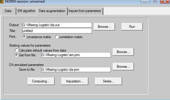
I suggest that you take the default settings for files. That means that the output of this procedure will be stored in a file named da.out and the starting values will come from the em.prm file, which is the output from the EM algorithm procedure. Now click on the Computing button and make sure that you are asking for at least 1000 imputations. Then click on the Imputations button and click the "impute at every kth iteration" and set k to 200. This means that the procedure will run through 1000 imputations and after each 200th imputation it will print out an imputed data set. Notice that the named imputed data set happens to be the name of our original data file, BUT with the extension .imp1 up to .imp5. Now click OK and then Run. The printout from that step is not very exciting, but now you have 5 new data sets.

Here is where you have to get to work. Set norm.exe aside, though you don't have to close it, and get out a program that will run logistic regression. (I am using SPSS because I have already set up the code for that.) What we are going to do is to run a regression on each of the five data sets, write out the regression coefficients and their standard errors from each run, record those values in a new data file, and then go back to norm to do the averaging.

I ran the logistic regression procedure on each imputation. I then created a file that contained
regression coefficients set 1
st. err set 1
regression coefficients set 2
st. err set 2
etc.
This file looked like

1.381470 -0.07461805 -2.106338 0.1347733  0.005269371
0.7840112 0.01374915  1.004061 0.04789091 0.04548990
1.264204 -0.07219109 -2.039125 0.1666566 -0.025356212
0.7648291 0.01346333  1.009399 0.05028284 0.04268443
1.546320 -0.08588102 -2.644697 0.1685393 -0.002134871
0.7897314 0.01667789  1.064713 0.05625988 0.04636413
1.199429 -0.08544579 -2.360542 0.1566628  0.023835288
0.8586487 0.01643126  1.095847 0.05081372 0.04424264
1.499090 -0.08318284 -2.337357 0.1404035  0.018431084
0.8111881 0.01559692  1.077959 0.05174125 0.04481766

This is ready for the next step. Now go to the norm.exe menu and select Analyze/MI Inference: Scalar.

Select the name of the data file. In my case it was called LogisticResults.dat. Now specify the number of estimands, which is the number of columns in this file. In our case there is an intercept and four predictors, so I enter "5". Clicking "Run" gives me the following output.

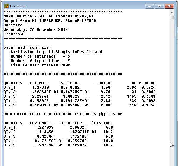
You can translate Qty_1 ... QTY_5 to "Intercept, survrate, gsi, avoid, and intrus." The regression coefficients are given in column 2, their standard errors in column 3, and a t test on each in column 4. The optimal regression equation using norm.exe is now

Ŷ = 1.378 - 0.080 * survrate - 2.298 * gsi + 0.153 * avoid + 0.004 * intrus

Compare these results with what we found with SPSS and with SAS. Those are repeated below.

Ŷ = 1.312 - 0.089 * survrate - 2.477 * gsi + 0.194 * avoid - 0.006 * intrus

Compare this with the result that we found with SAS, which follows.

Ŷ = -1.251 + 0.088 * survrate + 2.555 * gsi - 0.189 * avoid - 0.005 * intrus

I would say that we have a remarkable level of agreement, which is very nice to see.

References

Allison, P. D. (2001) Missing Data Thousand Oaks, CA: Sage Publications.Return

Barladi, A. N. &s; Enders, C. K. (2010). An introduction to modern missing data analyses. Journal of School Psychology, 48, 5-37.Return

Cohen, J. & Cohen, P. (1983) Applied multiple regression/correlation analysis for the behavioral sciences (2nd ed.).Hillsdale, NJ: Erlbaum. Return

Cohen, J. & Cohen, P., West, S. G. & Aiken, L. S. (2003). Applied Multiple Regression/Correlation Analysis for the Behavioral Sciences, 3rd edition. Mahwah, N.J.: Lawrence Erlbaum. Return

Dunning, T., & Freedman, D.A. (2008) Modeling section iffects. in Outhwaite, W. & Turner, S. (eds) Handbook of Social Science Methodology. London: Sage. Return

Howell,D. C. (2007) The analysis of missing data. In Outhwaite, W. & Turner, S. Handbook of Social Science Methodology. London: Sage.Return

Little, R.J.A. & Rubin, D.B. (1987) Statistical analysis with missing data. New York, Wiley. Return

Jones, M.P. (1996). Indicator and stratification methods for missing explanatory variables in multiple linear regression Journal of the American Statistical Association, 91,222-230. Return

Schafer, J. L. (1997). Analysis of incomplete multivariate data, London, Chapman & Hall.">

Schafer, J.L. & Olsden, M. K.. (1998). Multiple imputation for multivariate missing-data problems: A data analyst's perspective. Multivariate Behavioral Research, 33, 545-571.Return

Scheuren, F. (2005). Multiple imputation: How it began and continues. The American Statistician, 59, : 315-319.Return

Sethi, S. & Seligman, M.E.P. (1993). Optimism and fundamentalism. Psychological Science, 4, 256-259. Return

Last revised 6/25/2015