The question of mediated and moderated relationships has become an important one in psychology in recent years. The issue was popularized many years ago by Baron and Kenny (1986) in an article in the Journal of Personality and Social Psychology, and that is the classic reference. The use of this technique has continued to be important.
Baron and Kenny distinquished between the situation in which variable B serves a mediating role between variables A and C, and situations in which variable B moderates (or alters) the relationship between A and C. Let's start with an example. If we thought that the relationship between Intelligence and Income was due to the fact that Intelligence is associated with more Education, and that more Education leads to higher Income, then we would label Education as a mediating variable. At the same time, if we assumed that this relationship between Education and Income held for men, but, because of the ills of our society, it did not hold for women, then we would say that the Education --> Income relationship was moderated by Sex.
The example that I will use is built very directly on an excellent study by Kliewer, Lepore, Oskin, & Johnson (1998) on "The role of social and cognitive processes in children's adjustment to community violence." The study was published in The Journal of Consulting and Community Psychology. I have created data which match their data almost exactly, although I have not rounded my variables to integers, and each of the variables was drawn from a normal population before being transformed to have the reported means, standard deviations, and correlational structure of Kliewer et al's study. I have appended the SPSS syntax that created this file to the end of this page. The raw data file can be found at Kliewer.dat
A more recent and excellent example is a study by Russell, Ickes, & Ta, (2018) entitled "Women interact more comfortably and intimately with gay men - but not straight men - after learning their sexual orientation.Psychological Science, 29, 288-303. The study illustrates both mediation and moderation. I did not use it here because I was not able to generate the necessary data, but the raw data on individual variables are available as supplemental material.
Kliewer et al (1998) studied the relationship between the violence that a child observes or experiences directly and subsequent internalizing problems. They hypothesized that this particular relationship was mediated by the occurrence of intrusive thoughts, such that violence led to intrusive thoughts, which in turn led to internalizing behaviors. Furthermore, they hypothesized that this relationship was itself moderated by the social support and social strains impinging on the child. With considerable support and few strains, the violence that the child witnessed would not lead to a high level of intrusive thoughts, and those intrusive thoughts would not lead to internalizing problems. On the other hand, for those children with little social support and a high level of social strains, the violence → intrusive thoughts → internalizing paths would be strong. Kliewer et al. diagrammed this situation as:
In this diagram the top line represents a mediating set of relationships, while the vertical arrows represent moderating effects.
Variables:
Kliewer et al. collected data from 40 male and 59 female children aged 8-12 living in moderate- to high-violence areas of Richmond, VA. Data were collected from the children and their caregivers on 10 variables. These variables were
1) Witness violence        2) Victim of violence        3) Intrusive thoughts
4) Internalizing symptoms  5) Social support            6) Social strains
7) Current stress          8) Maternal education        9) Child age
10) Child sex
The data set contains all of these variables. However for our purposes I will only use some of them.
Results:
The descriptive statistics on all variables follows. These statistics are exactly equal to those obtained by the authors.
Mediating Relationships:
Descriptive Statistics
n
minimum
maximum
mean
std. deviation
age
99
7.52
13.67
10.7100
1.2700
gender
99
1.00
2.00
1.5960
.4932
id
99
1.00
99.00
50.0000
28.7228
internal
99
-7.02
4.89
6.2e-17
2.3500
intrus
99
2.25
20.64
10.0900
3.3200
mateduc
99
6.99
17.04
11.7500
1.9100
socsupp
99
15.56
41.91
27.5500
5.2500
sostrain
99
.09
8.56
3.7700
1.7000
stress
99
-2.14
7.29
2.9400
2.1200
violvict
99
-13.01
12.53
5.5404
????
violwit
99
-4.81
52.83
20.3600
12.4800
valid n (listwise)
I can't fit the SPSS printout in, so I'll simply copy the original matrix of correlations.
1 2 3 4 5 6 7 8 9 10 1) ViolWit 1.00 .43 .37 .20 .08 .19 .05 -.18 .20 -.20 2) ViolVict 1.00 .48 .31 -.04 .17 -.02 -.03 .04 -.05 3) Intrus 1.00 .39 -.08 .27 .04 -.25 -.09 .10 4) Internal 1.00 -.17 .33 .27 -.21 -.16 -.04 5) SocSupp 1.00 -.29 -.08 .12 .07 .06 6) SoStrain 1.00 .00 -.19 -.10 .09 7) Stress 1.00 .01 .06 -.08 8) MatEduc 1.00 .04 .01 9) Age 1.00 .00 10) Gender 1.00 Correlations > .20 are significant at p < .05
There is a lot to see in this table, but I'm going to focus on those relationships which relate directly to Kliewer's model. The authors included additional control variables (demographic variables and stress) in their model, but I will leave them out except for a demonstration after the next topic.
Does Violenct Predict Internalizing Symptoms?
Note that, as hypothesized, the correlation matrix shows a relationship between witnessing violence and later internalizing symptoms. The correlation (r = .20) was significant at p < .05. Thus we can conclude that there is a linear relationship between the degree to which children witness violence, and their level of internalizing symptoms. Whether or not this is a direct causal relationship is the next question.
Do Intrusive Thoughts Mediate the Violence → Internalizing Relationship?
Note that witnessing violence is significantly related to intrusive thoughts (r = .37), and that intrusive thoughts are related to Internalizing behaviors (r = .39). These significant relationships are required before we can test a mediating model. If they don't hold, then we can't have mediation. If they do hold, we can then ask if perhaps witnessing violence leads to an increase in intrusive thoughts, which, in turn, leads to an increase in internalizing symptoms.
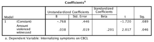
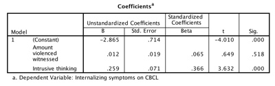
Suppose that we use both Witnessing violence and Intrusive thoughts as predictors of Internalizing behaviors. If Intrusions mediate the relationship between witnessing violence and internalizing behaviors, then the direct violence → Internal path should be drastically reduced when intrusions are added to the equation. The results follow, using just ViolWit as a predictor in the first model and ViolWit & Intrus in the second model.
Click on triangle to see (or hide) code and results in R
setwd("~/Dropbox/Webs/StatPages/Mediated-Moderated")
dat <- read.table("Kliewer.dat", head = TRUE)
attach(dat)  # Just for efficiency, but a poor idea

model1 <- lm(Internal ~ ViolWit)
summary(model1)
model2 <- lm(Internal ~ ViolWit + Intrus)
summary(model2)
_______________________________________________________________________________
model1 <- lm(Internal ~ ViolWit)

Coefficients:
            Estimate Std. Error t value Pr(>|t|)
(Intercept) -0.76762    0.44633  -1.720   0.0887 .
ViolWit      0.03775    0.01871   2.017   0.0464 *
---
Signif. codes:  0 ‘***’ 0.001 ‘**’ 0.01 ‘*’ 0.05 ‘.’ 0.1 ‘ ’ 1

Residual standard error: 2.312 on 97 degrees of freedom
Multiple R-squared:  0.04026,	Adjusted R-squared:  0.03036
F-statistic: 4.069 on 1 and 97 DF,  p-value: 0.04645
____________________________________________________

Model2

model2 <- Internal ~ ViolWit + Intrus)

Coefficients:
            Estimate Std. Error t value Pr(>|t|)
(Intercept) -2.86487    0.71436  -4.010 0.000120 ***
ViolWit      0.01232    0.01898   0.649 0.517671
Intrus       0.25906    0.07132   3.632 0.000453 ***
---
Signif. codes:  0 ‘***’ 0.001 ‘**’ 0.01 ‘*’ 0.05 ‘.’ 0.1 ‘ ’ 1

Residual standard error: 2.179 on 96 degrees of freedom
Multiple R-squared:  0.1562,	Adjusted R-squared:  0.1386
F-statistic: 8.887 on 2 and 96 DF,  p-value: 0.0002876
Notice that when ViolWit is used alone, it is a significant predictor, with β = .20, t = 2.01, and p = .047. (We already knew this from the intercorrelation matrix.) However when we add Intrus as a predictor, ViolWit is no longer significant, although Intrus is. This is the evidence we seek that intrusive thinking is the mediator in the ViolWit → Intrus relationship. This is a perfect example of Baron and Kenny's description.
We would find a similar relationship if we used the degree to which the child was a victim of violence, in place of just witnessing violence, but I will not show that here.
It is important to note that just because we have the pattern of relationships shown above, does not mean that intrusive thoughts mediate the relationship. We have met the statistical requirement, but that doesn't mean the logical requirement. Suppose, for example, that Intrus was measured a year before the child saw any violence. Then it would have been logically impossible for Intus to work as a mediator, even if the pattern of correlations were exactly the same. To demonstrate mediation you need to be able to make a logical argument about the relationship, as well as to show that it exhibits particular statistical properties. I would assume that for our particular case here, a logical argument can be made as well.
Conclusion:
So far, we have shown that simplying witnessing violence is sufficient to lead children to show internalizing behaviors. We have also shown that this relationship is mediated through intrusive thoughts.
Controlling Other Variables in a Mediating Model:
The preceding discussion is at a very simple level with only two variables. We can extend it to include a situation where we have additional variables that need to be considered, even if they are somewhat tangential to the direct mediating relationship. Suppose that we think that to fully understand the above relationship, we need to also control for demographic variables and concurrent life stress. The child's gender, his or her age, and the level of stress under which he or she generally lives should certainly be related to the level of internalizing behaviors, and we want to take these into account.The only difference in how we test our model is that we will include those variables at the first stage in the model, along with ViolWit.
These results follow:
Toggle triangle to show and hide R Code and results.
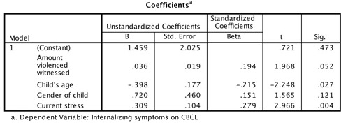
model3 <- lm(Internal ~ ViolWit + Age + gender + Stress)
model4 <- lm(Internal ~ ViolWit + Age + Gender + Stress + Intrus)
summary(model3)
summary(model4)
anova(model3, model4)
corr(ViolWit, Intrus, Gender, Age, Intrus)
___________________________________________________________

lm(formula = Internal ~ ViolWit + Age + Gender + Stress)

Coefficients:
            Estimate Std. Error t value Pr(>|t|)
(Intercept)  1.45936    2.02489   0.721  0.47288
ViolWit      0.03649    0.01854   1.968  0.05201 .
Age         -0.39764    0.17688  -2.248  0.02691 *
Gender       0.72008    0.46016   1.565  0.12098
Stress       0.30855    0.10403   2.966  0.00382 **

Residual standard error: 2.176 on 94 degrees of freedom
Multiple R-squared:  0.1767,	Adjusted R-squared:  0.1416
F-statistic: 5.042 on 4 and 94 DF,  p-value: 0.001002


lm(formula = Internal ~ ViolWit + Age + Gender + Stress + Intrus)

Coefficients:
            Estimate Std. Error t value Pr(>|t|)
(Intercept) -1.04308    2.08486  -0.500  0.61804
ViolWit      0.01444    0.01899   0.760  0.44889
Age         -0.30317    0.17136  -1.769  0.08014 .
Gender       0.55108    0.44230   1.246  0.21592
Stress       0.29656    0.09935   2.985  0.00362 **
Intrus       0.22237    0.06956   3.197  0.00190 **

Residual standard error: 2.076 on 93 degrees of freedom
Multiple R-squared:  0.2582,	Adjusted R-squared:  0.2183
F-statistic: 6.473 on 5 and 93 DF,  p-value: 3.314e-05

anova(model3, model4)
Analysis of Variance Table

Model 1: Internal ~ ViolWit + Age + Gender + Stress
Model 2: Internal ~ ViolWit + Age + Gender + Stress + Intrus
  Res.Df    RSS Df Sum of Sq      F   Pr(>F)
1     94 444.95
2     93 400.89  1    44.057 10.221 0.001898 **
Notice that we have the same pattern of results for the two important variables. In the third model, violWit is nearly significant, with β = .194, t = 1.97, and p = .052. This is even after we control for the other variables, two of which are sigificant.
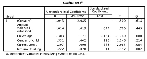
When we add Intrus to the model, ViolWit drops to a β = .077, t = ..760, p = ..449, while Intrus is significant, with β = .328, t = 3.326, and p = .001. Again, Age and Stress are also significant. So, again, we have shown the mediating role of intrusive thoughts.
I have reported beta in each of these analyses, because that is what you normally see as the path coefficient in the model. I won't go into that issue here because of time, other than to show the model as many people would report it.
Moderating Relationship
Moderating relationships are somewhat more complicated to see, although the calculations are not difficult. If you consider what I have suggested above, which is that the relationship between ViolWit and Intrus will depend upon whether or not the child has strong social support, you will realize that I am talking about what you normally think of as an interaction. Furthermore, you know that an interaction between two variables (A and B) is normally written as A × B, which is really a notation for multiplication. You may also know from elsewhere that we can get the interacting effects of two independent variables just by computing a new variable that is the product of the two separate variables. Thus if A and B were variables in our model, we could add their interaction by predicting Y from A, B, A ×B. That is what we will do here, although we will add a little twist.
As suggested, we could create our interaction variable by multiplying our two independent variables together. We could then use that product as a predictor along with the other two variables. The two independent variables would be the equivalent of main effects, and the product would carry information about the interaction. While this would be a legitimate way of testing for an interaction, we would be likely to find that the product of A and B is highly correlated with A or B or with both. This leads to problems with collinearity, and makes the tests on main effects problematic.
An alternative approach is to "center" each of the main effect variables by subtracting their respective means from all observations. We could then form a product of these centered variables, and it would be only weakly correlated to either of them (or with their non-centered counterparts). This approach is often taken, but there is a slightly simpler way that leaves us at the same place. We can simply standardize A and B and then calculate the product of zA and zB. This product will do just as well as the product of centered variables. (I say it is simpler because SPSS will do it automatically through Statistics/Summarize/Descriptives
The following printout has used the main effects of ViolWit and social strain (SoStrain), as well as the product of their standardized values. We could have used the standardized values of ViolWit and SoStrain as our main effects, but the results would have been the same except that the slopes would reflect the different values of the standard deviations of the variables. The t tests on the slopes would have been unaffected, however.
(You might wonder why I switched from social support to social strain. It's really just because I liked the results better, and when you're making up an example, it's nice to have nice results--even if they aren't as nice as I would like.)

Toggle triangle to show and hide R Code and results.
### These results differ from SPSS, at least in part because the SPSS program below
### generates random data each time it runs.
###Mediation

setwd("~/Dropbox/Webs/StatPages/Mediated-Moderated")
dat <- read.table("Kliewer.dat", head = TRUE)
attach(dat)  # Just for efficiency, but a poor idea
SocStrain <- SosTrain    # Just to correct a dumb spelling error

model1 <- lm(Internal ~ ViolWit)
summary(model1)
model2 <- lm(Internal ~ ViolWit + Intrus)
summary(model2)

model3 <- lm(Internal ~ ViolWit + Age + Gender + Stress)
model4 <- lm(Internal ~ ViolWit + Age + Gender + Stress + Intrus)
summary(model3)
summary(model4)
anova(model3, model4)


### First center the variables -- I have standardized them
centeredData <- as.data.frame(scale(dat, center = TRUE))
describe(centeredData)
model5 <- lm(Internal ~ ViolWit + SocStrain + ViolWit*SocStrain, data = centeredData)
summary(model5)
_____________________________________________________________________

lm(formula = Internal ~ ViolWit + SocStrain + ViolWit * SocStrain,
    data = centeredData)

Coefficients:
                  Estimate Std. Error t value Pr(>|t|)
(Intercept)       -0.66780    0.23632  -2.826  0.00575 **
ViolWit            0.20475    0.26453   0.774  0.44086
SocStrain          0.17868    0.05757   3.104  0.00252 **
ViolWit:SocStrain -0.01631    0.06521  -0.250  0.80299

Residual standard error: 0.9481 on 95 degrees of freedom
Multiple R-squared:  0.1286,	Adjusted R-squared:  0.1011
F-statistic: 4.674 on 3 and 95 DF,  p-value: 0.00433
These results are not quite what I woould like. Notice that they illustrate that both ViolWit and SoStrain contribute to the prediction of Intrusive thoughts. However the interaction term is nowhere near significant. I will need to find a better dataset.
Standardized Witness Violence
Standardized Social Strain -2 0 2 -2 3.93 8.75 13.56 0 8.01 10.21 12.41 2 12.10 11.68 11.26 Along the top of the table I have three different representative values for ViolWit. Down the left of the table of I have three different representative values for Social Strain. (Both of these variables are in their standardized form.) The entries in the table are the predicted value of Intrusive thoughts given the model in the previous table. For example, 1.1(-2) + .733(-2) - .654(-2)(-2) + 10.213 = 3.93.
Notice that children who have very high levels of social strain are at high levels of instrusive thoughts no matter how much violence they witness. But children who don't have much social strain only show high levels of instrusive thoughts if they witness a lot of violence. Otherwise, they have low levels of intrustive thoughts. In other words, the effect of ViolWit depends on the level of social strain. This is what we mean by an interaction. It is also what we mean by a moderating effect of social strain.
I must admit that this last paragraph doesn't sound quite like the theory that I developed in the beginning, although that theory was specifically aimed as social support more than social strain. I would be happier if the prediction for low values of SoStrain remained low at all levels of ViolWit, but you can't have everything. What I have said is accurate, but it doesn't fit neatly together.
You might do well to play with these data. You could replace social strain with social support, and you would see that with high levels of social support, witnessing violence in not that much different from not witnessing it, as far as intrusive thoughts are concerned. But with low levels of social support, witnessing violence has a major effect on intrusive thoughts. You could also investigate the effects of controlling demographic and stress variables.
SPSS Syntax
There is much more that could be made of these data, and I encourage student to play with them.
The following code is for SPSS. You can simply copy it and paste it into an SPSS syntax file.
*  This program generates a set of data which have been drawn from
*  populations having the pattern of correlations specified in
*  "compute r = { }" below. If you run a principal components analysis
*  and extract all factors, and enter these factors in the
*  matrix statements (in place of r1, r2, ...), the output variables
*  will have exactly the pattern of correlations given in r.
*  Written by: David C. Howell
*  The factor commands were supplied by Lawrence Gordon.
*  last updated: 4/27/98
new file.
input program.
*  draw 99 cases.
set seed 3458769.
loop i = 1 to 99.
*  draw data for 10 variables.
do repeat response = r1 to r10.
compute response = rv.normal(0,1).
end repeat.
end case.
end loop.
end file.
end input program.
* modify the next line for your own system.save outfile = "dataout.sav".
* the next commands provide a principal components analysis and
* give orthogonal factors which will then reproduce the matrix exactly.
* you will have to modify in 3 places to adjust to the number of variables
* that you have in your example.
factor
/variables r1 to r10
/analysis r1 to r10
/print correlation extraction
/criteria factors(10) iterate(25)
/extraction pc
/rotation norotate
	/save reg(all).
	save outfile = "dataout.sav".

*  SPSS version 8.0 is very fussy about the matrix procedure which follows, and
*  seems to self-distruct, rather than leave a simple message, if you make the
*  slightest error. The easiest place for errors is in the correlation matrix.
*  After you have proofread it, profreed it two more times and then expect to correct
*  it again when the program fails.

    matrix.
	get x
	/file = "dataout.sav"
	/variables = fac1_1 to fac10_1.

compute r = {1.0, .43, .37, .20, .08, .19, .05, -.18, .20, -.20;
	.43, 1.0, .48, .31, -.04, .17, -.02, -.03, .04, -.05;
	.37, .48, 1.0, .39, -.08, .27, .04, -.25, -.09, -.10;
	.20, .31, .39, 1.0, -.17, .33, .27, -.21, -.16, -.04;
	.08, -.04, -.08, -.17, 1.0, -.29, -.08, .12, .07, .06;
	.19, .17, .27, .33, -.29, 1.0, .00, -.19, -.10, .09;
	.05, -.02, .04, .27, -.08, .00, 1.0, .01, .06, -.08;
	-.18, -.03, -.25, -.21, .12, -.19, .01, 1.0, .04, .01;
	.20, .04, -.09, -.16, .07, -.10, .06, .04, 1.0, .00;
	-.20, -.05, -.10, -.04, .06, .09, -.08, .01, .00, 1.0}.
compute newx = x*chol(r).
save newx /outfile = */variables = nr1 to nr10.
end matrix.
compute violwit = nr1*12.48+20.36.
compute violvict = nr2*2.43*2.28.
compute intrus = nr3*3.32+10.09.
compute internal=nr4*2.35 + 0.
compute socsupp=nr5*5.25+27.55.
compute sostrain=nr6*1.70+3.77.
compute stress=nr7*2.12+2.94.
compute mateduc=nr8*1.91+11.75.
compute age=nr9*1.27+10.71.
recode  (lowest thru -.24=1) (else=2) into gender .
execute .
save outfile = "dataout.sav"
  /drop nr1 to nr10.
correlations
	/variables=nr1 to nr10 /print=twotail sig.
David C. Howell
6/26/2015