Matplotlib basics

The basics of Matplotlib
We’re just going to cover the basics here. Why? Because Matplotlib has thousands of features and it has excellent documentation. So we’re just going to dip a toe in the waters.
For more, see:
- Matplotlib website: https://matplotlib.org
- Getting started guide: https://matplotlib.org/stable/users/getting_started
- Documentation: https://matplotlib.org/stable/index.html
- Quick reference guides and handouts: https://matplotlib.org/cheatsheets
The most basic basics
We’ll start with perhaps the simplest interface provided by Matplotlib, called pyplot. To use pyplot we usually import and abbreviate:
import matplotlib.pyplot as plt Renaming isn’t required, but it is commonplace (and this is how it’s done in the Matplotlib documentation). We’ve seen this syntax before—using as to give a name to an object without using the assignment operator (=). It’s very much like giving a name to a file object when using the with context manager. Here we give matplotlib.pyplot a shorter name plt so we can refer to it easily in our code. This is almost as if we’d written
import matplotlib.pyplot

plt = matplotlib.pyplot
Almost.
Now let’s generate some data to plot. We’ll generate random numbers in the interval (-1.0, 1.0).
import random

data = [0]
for _ in range(100):
    data.append(data[-1]
                + random.random()
                * random.choice([-1, 1]))
So now we’ve got some random data to plot. Let’s plot it.
plt.plot(data)That’s pretty straightforward, right?
Now let’s label our y axis.
plt.ylabel('Random numbers (cumulative)')Let’s put it all together and display our plot.
import random
import matplotlib.pyplot as plt

data = [0]
for _ in range(100):
    data.append(data[-1]
                + random.random()
                * random.choice([-1, 1]))
plt.plot(data)
plt.ylabel('Random numbers (cumulative)')
plt.show()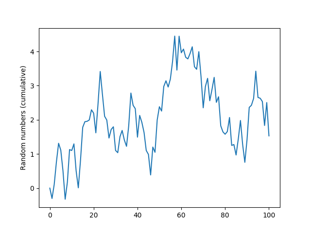
It takes only one more line to save our plot as an image file. We call the savefig() method and provide the file name we’d like to use for our plot. The plot will be saved in the current directory, with the name supplied.
import random
import matplotlib.pyplot as plt

data = [0]
for _ in range(100):
    data.append(data[-1]
                + random.random()
                * random.choice([-1, 1]))

plt.plot(data)
plt.ylabel('Random numbers (cumulative)')
plt.savefig('my_plot.png')
plt.show()
That’s it. Our first plot—presented and saved to file.
Let’s do another. How about a bar chart? For our bar chart, we’ll use this as data (which is totally made up by the author):
| Flavor | Servings |
|---|---|
| Cookie dough | 9,214 |
| Strawberry | 3,115 |
| Chocolate | 5,982 |
| Vanilla | 2,707 |
| Fudge brownie | 6,553 |
| Mint chip | 7,005 |
| Kale and beet | 315 |
Let’s assume we have this saved in a CSV file called flavors.csv. We’ll read the data from the CSV file, and produce a simple bar chart.
import csv

import matplotlib.pyplot as plt

servings = []  # data
flavors = []   # labels

with open('flavors.csv') as fh:
    reader = csv.reader(fh)
    for row in reader:
        flavors.append(row[0])
        servings.append(int(row[1]))

plt.bar(flavors, servings)
plt.xticks(flavors, rotation=-45)
plt.ylabel("Servings")
plt.xlabel("Flavor")
plt.tight_layout()

plt.show()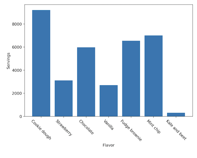
Voilá! A bar plot!
Notice that we have two lists: one holding the servings data, the other holding the x-axis labels (the flavors). Instead of plt.plot() we use plt.bar() (makes sense, right?) and we supply flavors and servings as arguments. There’s a little tweak we give to the x-axis labels, we rotate them by 45 degrees so they don’t all mash into one another and become illegible. plt.tight_layout() is used to automatically adjust the padding around the plot itself, leaving suitable space for the bar labels and axis labels.
Be aware of how plt.show() behaves
When you call plt.show() to display your plot, Matplotlib creates a window and displays the plot in the window. At this point, your program’s execution will pause until you close the plot window. When you close the plot window, program flow will resume.
Summary
Again, this isn’t the place for a complete presentation of all the features of Matplotlib. The intent is to give you just enough to get started. Fortunately, the Matplotlib documentation is excellent, and I encourage you to look there first for examples and help.
Copyright © 2023–2025 Clayton Cafiero
No generative AI was used in producing this material. This was written the old-fashioned way.