Elementary statistics

Published

2023-07-31

Some elementary statistics

Statistics is the science of data—gathering, analyzing, and interpreting data.

Here we’ll touch on some elementary descriptive statistics, which involve describing a collection of data. It’s usually among the first things one learns within the field of statistics.

The two most widely used descriptive statistics are the mean and the standard deviation. Given some collection of numeric data, the mean gives us a measure of the central tendency of the data. There are several different ways to calculate the mean of a data set. Here we will present the arithmetic mean (average). The standard deviation is a measure of the amount of variation observed in a data set.

We’ll also look briefly at quantiles, which provide a different perspective from which to view the spread or variation in a data set.

The arithmetic mean

Usually, when speaking of the average of a set of data, without further qualification, we’re speaking of the arithmetic mean. You probably have some intuitive sense of what this means. The mean summarizes the data, boiling it down to a single value that’s somehow “in the middle.”

Here’s how we define and calculate the arithmetic mean, denoted \mu, given some set of values, X.

\mu = \frac{1}{N} \sum\limits_{i \; = \;0}^{N - 1} x_i

where we have a set of numeric values, X, indexed by i, with N equal to the number of elements in X.

Here’s an example: number of dentists per 10,000 population, by country, 2020.¹

The first few records of this data set look like this:

Country	Value
Bangladesh	0.69
Belgium	11.33
Bhutan	0.97
Brazil	6.68
Brunei	2.38
Cameroon	0.049
Chad	0.011
Chile	14.81
Colombia	8.26
Costa Rica	10.58
Cyprus	8.58

Assume we have these data saved in a CSV file named dentists_per_10k.csv. We can use Python’s csv module to read the data.

data = []
with open('dentists_per_10k.csv', newline='') as fh:
    reader = csv.reader(fh)
    next(reader)  # skip the first row (column headings)
    for row in reader:
        data.append(float(row[1]))

We can write a function to calculate the mean. It’s a simple one-liner.

def mean(lst):
    return sum(lst) / len(lst)

That’s a complete implementation of the formula:

\mu = \frac{1}{N} \sum\limits_{i \; = \;0}^{N - 1} x_i

We take all the x_i and add them up (with sum()). Then we get the number of elements in the set (with len()) and use this as the divisor. If we print the result with print(f"{mean(data):.4f}") we get 5.1391.

That tells us a little about the data set: on average (for the sample of countries included) there are a little over five dentists per 10,000 population. If everyone were to go to the dentist once a year, that would suggest, on average, that each dentist serves a little less than 2,000 patients per year. With roughly 2,000 working hours in a year, that seems plausible. But the mean doesn’t tell us much more than that.

To get a better understanding of the data, it’s helpful to understand how values are distributed about the mean.

Let’s say we didn’t know anything about the distribution of values about the mean. It would be reasonable for us to assume these values are normally distributed. There’s a function which describes the normal distribution, and you’ve likely seen the so-called “bell curve” before.

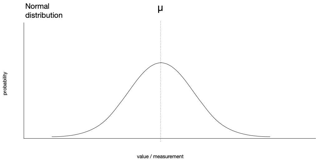
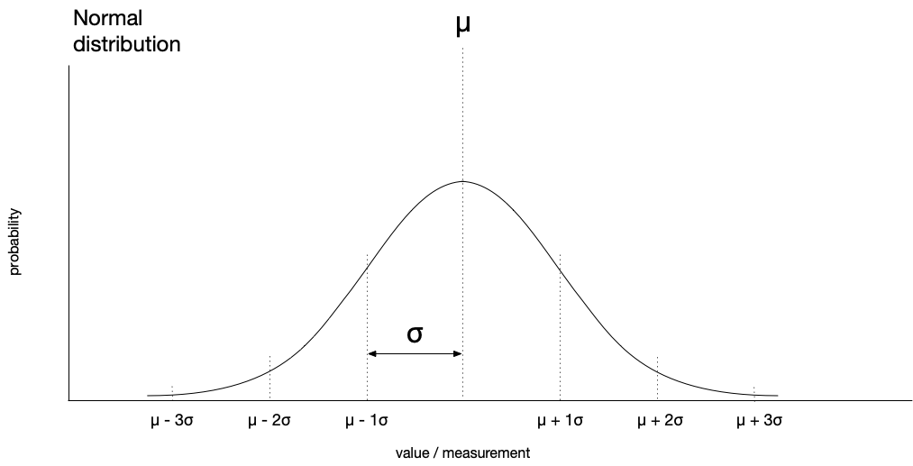
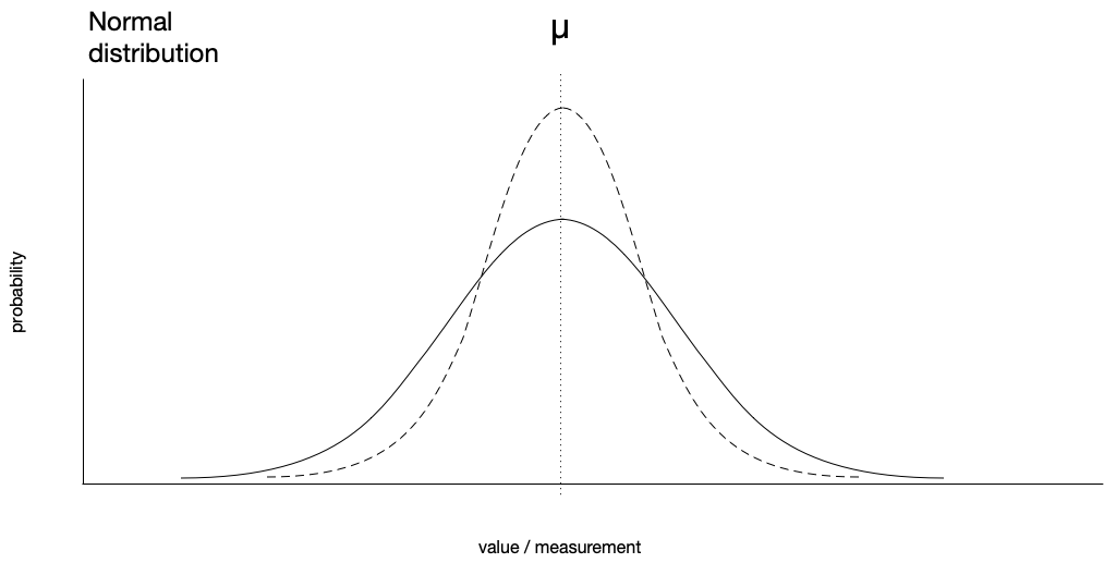
On the x-axis are the values we might measure, and on the y-axis we have the probability of observing a particular value. In a normal distribution, the mean is the most likely value for an observation, and the greater the distance from the mean, the less likely a given value. The standard deviation tells us how spread out values are about the mean. If the standard deviation is large, we have a broad curve:

With a smaller standard deviation, we have a narrow curve with a higher peak.

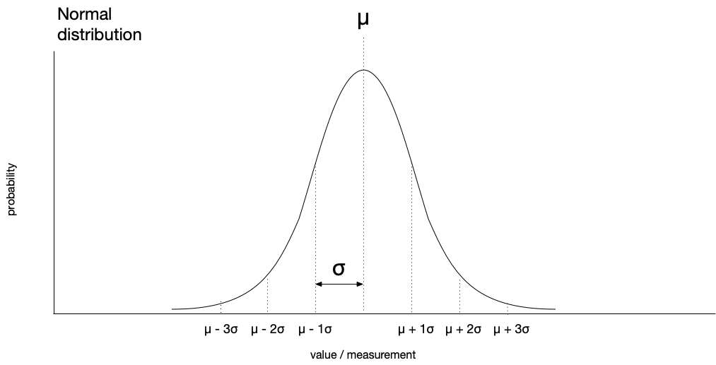
The area under these curves is equal.

If we had a standard deviation of zero, that would mean that every value in the data set is identical (that doesn’t happen often). The point is that the greater the standard deviation, the greater the variation there is in the data.

Just like we can calculate the mean of our data, we can also calculate the standard deviation. The standard deviation, written \sigma, is given by

\sigma =\sqrt{\frac{1}{N} \sum\limits_{i \; = \;0}^{N - 1} (x_i - \mu)^2}.

Let’s unpack this. First, remember the goal of this measure is to tell us how much variation there is in the data. But variation with respect to what? Look at the expression (x_i - \mu)^2. We subtract the mean, \mu, from each value in the data set x_i. This tells us how far the value of a given observation is from the mean. But we care more about the distance from the mean rather than whether a given value is above or below the mean. That’s where the squaring comes in. When we square a positive number we get a positive number. When we square a negative number we get a positive number. So by squaring the difference between a given value and the mean, we’re eliminating the sign. Then, we divide the sum of these squared differences by the number of elements in the data set (just as we do when calculating the mean). Finally, we take the square root of the result. Why do we do this? Because by squaring the differences, we stretch them, changing the scale. For example, 5 - 2 = 3, but 5^2 - 2^2 = 25 - 4 = 21. So this last step, taking the square root, returns the result to a scale appropriate to the data. This is how we calculate standard deviation.²

As we calculate the summation, we perform the calculation (x_i - \mu)^2. On this account, we cannot use sum(). Instead, we must calculate this in a loop. However, this is not too terribly complicated, and implementing this in Python is left as an exercise for the reader.

Assuming we have implemented this correctly, in a function named std_dev(), if we apply this to the data and print with print(f"{std_dev(data):.4f}"), we get 4.6569.

How do we interpret this? Again, the standard deviation tells us how spread out values are about the mean. Higher values mean that the data are more spread out. Lower values mean that the data are more closely distributed about the mean.

What practical use is the standard deviation? There are many uses, but it’s commonly used to identify unusual or “unlikely” observations.

We can calculate the area of some portion under the normal curve. Using this fact, we know that given a normal distribution, we’d expect to find 68.26% of observations within one standard deviation of the mean. We’d expect 95.45% of observations within two standard deviations of the mean. Accordingly, the farther from the mean, the less likely an observation. If we express this distance in standard deviations, we can determine just how likely or unlikely an observation might be (assuming a normal distribution). For example, an observation that’s more than five standard deviations from the mean would be very unlikely indeed.

Range	Expected fraction in range
\mu \pm \sigma	68.2689%
\mu \pm 2\sigma	95.4500%
\mu \pm 3\sigma	99.7300%
\mu \pm 4\sigma	99.9937%
\mu \pm 5\sigma	99.9999%

When we have real-world data, it’s not often perfectly normally distributed. By comparing our data with what would be expected if it were normally distributed we can learn a great deal.

Returning to our dentists example, we can look for possible outliers by iterating through our data and finding any values that are greater than two standard deviations from the mean.

m = mean(data)
std = std_dev(data)

outliers = []
for datum in data:
    if abs(datum) > m + 2 * std:
        outliers.append(datum)

In doing so, we find two possible outliers—14.81, 16.95—which correspond to Chile and Uruguay, respectively. This might well lead us to ask, “Why are there so many dentists per 10,000 population in these particular countries?”

Python’s `statistics` module

While implementing standard deviation (either for a sample or for an entire population) is straightforward in Python, we don’t often write functions like this ourselves (except when learning how to write functions). Why? Because Python provides a statistics module for us.

We can use Python’s statistics module just like we do with the math module. First we import the module, then we have access to all the functions (methods) within the module.

Let’s start off using Python’s functions for mean and population standard deviation. These are statistics.mean() and statistics.pstdev(), and they each take an iterable of numeric values as arguments.

import csv
import statistics

data = []
with open('dentists_per_10k.csv', newline='') as fh:
    reader = csv.reader(fh)
    next(reader)  # skip the first row
    for row in reader:
        data.append(float(row[1]))
    
print(f"{statistics.mean(data):.4f}")
print(f"{statistics.pstdev(data):.4f}")

When we run this, we see that the results for mean and standard deviation—5.1391 and 4.6569, respectively—are in perfect agreement with the results reported above.

The statistics module comes with a great many functions including:

mean()
median()
pstdev()
stdev()
quantiles()

among others.

Using the `statistics` module to calculate quantiles

Quantiles divide a data set into continuous intervals, with each interval having equal probability. For example, if we divide our data set into quartiles (n = 4), then each quartile represents 1/4 of the distribution. If we divide our data set into quintiles (n = 5), then each quintile represents 1/5 of the distribution. If we divide our data into percentiles (n = 100), then each percentile represents 1/100 of the distribution.

You may have seen quantiles—specifically percentiles—before, since these are often reported for standardized test scores. If your score was in the 80^th percentile, then you did better than 79% of others taking the test. If your score was in the 95^th percentile, then you’re in the top 5% all those who took the test.

Let’s use the statistics module to find quintiles for our dentists data (recall that quintiles divide the distribution into five parts).

If we import csv and statistics and then read our data (as above), we can calculate the values which divide the data into quintiles thus:

quintiles = statistics.quantiles(data, n=5)
print(quintiles)

Notice that we pass the data to the function just as we did with mean() and pstdev(). Here we also supply a keyword argument, n=5, to indicate we want quintiles. When we print the result, we get

[0.274, 2.2359999999999998, 6.590000000000001, 8.826]

Notice we have four values, which divide the data into five equal parts. Any value below 0.274 is in the first quintile. Values between 0.274 and 0.236 (rounding) are in the second quartile, and so on. Values above 8.826 are in the fifth quintile.

If we check the value for the United States of America (not shown in the table above), we find that the USA has 5.99 dentists per 10,000 population, which puts it squarely in the third quartile. Countries with more than 8.826 dentists per 10,000—those in the top fifth—are Belgium (11.33), Chile (14.81), Costa Rica (10.58), Israel (8.88), Lithuania (13.1), Norway (9.29), Paraguay (12.81), and Uruguay (16.95). Of course, interpreting these results is a complex matter, and results are no doubt influenced by per capita income, number and size of accredited dental schools, regulations for licensure and accreditation, and other infrastructure and economic factors.³

Other functions in the `statistics` module

I encourage you to experiment with these and other functions in the statistics module. If you have a course in which you’re expected to calculate means, standard deviations, and the like, you might consider doing away with your spreadsheet and trying this in Python!

Original author: Clayton Cafiero < [given name] DOT [surname] AT uvm DOT edu >

No generative AI was used in producing this material. This was written the old-fashioned way.

This material is for free use under either the GNU Free Documentation License or the Creative Commons Attribution-ShareAlike 3.0 United States License (take your pick).

Footnotes

Source: World Health Organization: https://www.who.int/data/gho/data/indicators/indicator-details/GHO/dentists-(per-10-000-population) (retrieved 2023-07-07)↩︎
Strictly speaking, this is the population standard deviation, and is used if the data set represents the entire universe of possible observations, rather than just a sample. There’s a slightly different formula for the sample standard deviation.↩︎
I’m happy with my dentist here in Vermont, but I will say she’s booking appointments over nine months in advance, so maybe a few more dentists in the USA wouldn’t be such a bad thing.↩︎

Some elementary statistics

The arithmetic mean

Python’s statistics module

Using the statistics module to calculate quantiles

Other functions in the statistics module

Footnotes

Python’s `statistics` module

Using the `statistics` module to calculate quantiles

Other functions in the `statistics` module